Abstract— The majority of researches on scheduling assume setup times negligible or as a part of the processing time. In this paper, job shop scheduling with sequence dependent setup times is considered. After defining the problem, a mathematical model is developed. Implementing the mathematical model in large problems presents a weak performance to find the optimum results in reasonable computational times. Although the proposed mathematical model presents a good performance to obtain feasible solutions, it is unable to reach the optimum results in larger problems. Thus, a heuristic model based on priority rules is developed. Because of the inability to find optimum solutions in reasonable computational times, 3 different innovative lower bounds are developed, which could be implemented to evaluate different heuristics and metaheuristics in large problems. The performance of the heuristic model evaluated with a well-known example in the literature insures that the model seems to have a strong ability to solve jobshop scheduling with sequence dependent setup times problems and to obtain good solutions in reasonable computational times.
Keywords: Job-shop scheduling, Heuristic model, , Priority rules, Mathematical model
I. INTRODUCTION
Scheduling problems exist almost everywhere in real industrial world situations. Scheduling involves determination of the order of processing a set of tasks on resources or machines. Job shop scheduling (JSS) problem involves an assignment of a set of tasks to the workstations (machines) in a predefined sequence in order to optimize one or more objectives considering job performances measures of the system. A job shop environment consists of
n job and each job has a given machine route in which some
machines can be missed and some can repeat [1]. Job shop scheduling (JSS) problem has been widely studied over the last four decades. Many researches involved job shop scheduling have been presented and various approaches have been implemented to solve this problem. Techniques such as Integer linear Programming were used in various researches such as [2] and [3]. Meta heuristics such as Tabu Search method [4], Genetic Algorithm [5] and Simulated Annealing [6] are widely used in recent years. Nevertheless, reviews of dispatching rules, which are variously used in the literature, have been presented in [7]. The dynamic
Manuscript received October 9, 2007.
1R.Moghaddas, Department of Industrial Engineering, Sharif University
of Technology, Azadi Street, Tehran, Iran.
(Phone: +98-0935- 848-0502; Fax: +98-021-66820392; e-mail:[email protected]).
2M.Houshmand, Associate Professor, Department of Industrial
Engineering, Sharif University of Technology, Azadi Street, Tehran, Iran. (Phone: +98-0912-104-2244; e-mail: [email protected]).
scheduling problem (DJSSP) could be considered as a queuing system that consists of machines and jobs where each job requires a specified sequence (routing) on the machines and involves certain amount of processing time. The dynamic job shop scheduling problem (DJSSP) addressed in this paper involves deciding the priority for the jobs waiting to be processed considering desired objectives. One of the real conditions that industry usually confronts with is setup consideration. The setup time has been considered negligible for long time and entered the problems as a part of the processing time. The importance and applications of scheduling models considering setup times (costs) have been discussed in several researches since the mid-1960s [1]. In this paper, we consider the typical case, which is called sequence-dependent setup times, where the setup time depends on the job previously processed on each machine. Hence, there are matrices for each machine that represent the relationships between jobs that have at least one operation on that machine. [8] and [9] presents a comprehensive review of scheduling research in which the setup time or cost is considered. [9] classifies scheduling problems into batch and non-batch, sequence-independent and sequence-dependent setup, and categorizes the literature according to the shop environments of single machine, parallel machines, flow shops, and job shops. [1] aims to provide an extensive review of the scheduling problems, which considers the setup times (costs). That paper mentioned that during 1999 to 2006, there has been a significant increase in interest in scheduling problems involving setup times (costs).
Various approaches such as Heuristic algorithms [10], Simulation [11], Branch and Bound algorithm ([12], [13]), Integer Programming ([14], [15], [16]) and Genetic Algorithm ([17], [18]), are implemented to solve job shop scheduling with sequence dependent setup times. Among these papers, Cmax (makespan) which is the maximum total completion time of all jobs is implemented more than other performance criteria and sequence dependent setup times are considered in most of them.
The job shop-scheduling problem is widely acknowledged as one of the most difficult NP-complete problems ([19], [20]) that might not have good efficiency to find the optimum result of large problems in reasonable computational times. Usually, these problems are considered as combinatorial optimization problems and difficult-to-solve because of extremely complicated constraints [21]. Sequence-dependent scheduling problems are one of the most difficult classes of scheduling problems [22] and as Sequence Dependent Setup Times Job Shop Scheduling Problem is an extension of job-shop scheduling which all setup times are equal to zero, it is NP-hard as well, justifying the use of heuristics or approximation algorithms.
Job-Shop Scheduling Problem With
Sequence Dependent Setup Times
In this paper, an innovative mixed-integer linear programming using Traveling Salesman Problem (TSP) is presented. In addition, before defining the mathematical model, some steps are proposed in order to have a model with fewer constraints and variables. The objective is to minimize the makespan, which aims at reducing the completion time of the final job. Finally, a heuristic search procedure, which is based on a new innovative rule, is presented. Both mathematical programming and the heuristic procedures are implemented in one of the well – known example in the literature and the results will be analyzed. In order to evaluate the heuristic and metaheuristic algorithms, which are implemented in large problems, three different lower bounds are developed in this paper. These lower bounds considering setup times will be efficient in job shop scheduling with sequence dependent setup times.
II. THEMODEL
A. Assumptions
The shop environment considered in this paper consists of scheduling a set of n jobs that need to be processed by a set
of m machines. The main assumptions of the presented
model are described as follows:
1) Every job has a unique sequence on m machines. There
are no alternate routings.
2) There is only one machine of each type in the shop. 3) Processing times for all jobs are known and constant. 4) All jobs are available for processing at time zero. However, because of the flexibility of the decision variables, if there are some jobs or operations available later than time zero in the shop floor, the related constraint could be easily added to the model.
5) The setup times of jobs on each machine are sequence dependent and are known. These setup times are available for each kind of machines. Hence, the setup matrix for all machines is generated just for the operations, which require the same machine.
6) Each machine can perform only one operation at a time on any job.
7) An operation of a job can be performed by only one machine.
8) Once an operation has begun on a machine, it must not be interrupted. Process pre-emption is not allowed.
9) An operation of a job cannot be performed until its preceding operations are completed.
8) Each machine is continuously available for production; hence, there are no machine breakdowns.
10) There is no restriction on queue length for any machine. 11) There are no limiting resources other than machines/workstations.
12) The machines are not identical and perform different operations.
The objective is to minimize the makespan, denoted by Cmax, referring to the latest completion time of the jobs. Note that, if a job passes a machine more than once and if there is an assembly requirement in shop floor, both heuristic and mathematical models could cover these constraints.
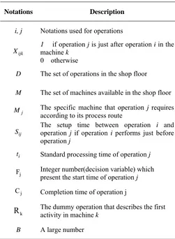
[image:2.595.299.550.83.425.2]The following table describes the notations used in the model:
Table 1: Notations of the mathematical model
Notations Description
i, j Notations used for operations
ijk
X
1 if operation j is just after operation i in the
machine k
0 otherwise
D The set of operations in the shop floor
M The set of machines available in the shop floor j
M The specific machine that operation j requires according to its process route
ij
S
The setup time between operation i and
operation j if operation i performs just before
operation j i
t Standard processing time of operation j
j
F Integer number(decision variable) which present the start time of operation j
j
C Completion time of operation j
k
R
The dummy operation that describes the first activity in machine kB A large number
It should be mentioned that TSP is implemented in order to define the decision variables. TSP is a typical combinatorial optimization problem, that a salesman is required to visit cities exactly for once with minimum distances. The followings are the assumptions of a TSP model that corresponds to the job shop scheduling problem with sequence dependent setup times:
1. The salesman visits every city exactly once. In applying TSP in job-shop scheduling (JSS), each operation of a job is considered as a city. Furthermore, the path that salesman visits through his tour, is the sequence of operations on each machine. Note that setup times are the distances between the cities.
2. In TSP the salesman starts from a known city and finish his tour in that city. In job-shop scheduling, the start of the sequences are unidentified. In order to reach this condition, a dummy activity is defined in order to discriminate the starting operation of each machine. Note that the operation of this variable eliminates all subtours. In this model, there are not any extra variables existed in the model in order to eliminate subtours.
B. Mathematical Model
job i, operation j is equal to
i
×
m
+
j
, which m is the totalnumber of available machines in the shop floor. The mathematical model is described as follows:
(1) D i∈ ) (
max Ci Fi ti
makespan
Min = = +
Subject to:
(2) 1
=
∑
i∈DXijk) |
, (
, j k k Mi Mj
D
j∈ = =
(3) 1
=
∑
j∈DXijk
) |
, (
, i k k Mi Mj
D
i∈ = =
(4) ) 1 ( ijk j ij i
i t S F B X
F + + <= + × −
) | , , ( , ) ,
(i j ∈D i j k k=Mi=Mj
(5)
ij
S j i, ∈
j i
i t F
F + <= (6) M k∈ o t k R = (7) ) | , (
, i k k Mi
D
i∈ =
0
, =
=
k ki iR
R o S
S
Equation (1) presents the objective function, which aims to reduce the cycle time of all jobs called makespan. Constraint 2 and constraint 3 force the job scheduling to have a unique sequence in a schedule sequence of each machine. Constraint 4 requires that the start time of each operation in one machine should be larger than the completion time of the operation that performs just before this operation considering the setup times between the pervious operation and current operation. Constraint 5 ensures that an operation could not start until its preceding operation is done. In constraint 6 and constraint 7, processing time and the relationship of setup times between dummy operations and other operations, which require the same machine, are set to zero. The existence of variable Fi in the mathematical model eliminates the subtours in the solutions. It should be noted that the operation, which starts in the next location after dummy operation of a machine, is the starting point of sequence and consequently no setup is required to perform this operation. Note that, if any operation of a job, pass each machine more than once, the related constraint could be easily added to the model with some modification to constraint 5 considering the precedence constraints.
Nevertheless, if some jobs (operations) arrive at the shop floor later than time zero, the following constraint could be added to the model:
i
i F
A <= (8) Note that Ai is the arrival time of operation i in the shop
floor. In this model, it is assumed that each setup processing does not require jobs to start on each machine. Hence, the setup times could start on each machine even if that job is not available in the current machine yet. In this paper, other type of setup that the setup requires the presence of the job is also considered. The following constraint is added to model in order to cover this assumption:
j k
M
z zj zjk
i
i t S X F
F z <= × + +
∑
= ) |( (9) )
| , ,
(i jk Mi =Mj =k
In order to evaluate the efficiency of the proposed model, its efficiency is tested with various well-known examples. Most
of the studies in the literature have used between four and 10 machines. In this paper one well known problem (20-job 5-machine problem from [23] is selected and with some modification, 10 instances were generated to evaluate the efficiency of the model. The setup times are randomly generated according to the uniform discrete distribution
U[0, min ti]( high variability) and U[0,.5* min ti]( low variability) which ti is the processing time of the operations of each machine. The final instances have setup matrixes for each machine. The computational time for evaluating the mathematical model is set to 3600 seconds which implemented by Pentium 4 with 256 Mb RAM using LINGO 10. The result of implementing the model in various
problems ensures that where the number of machine and jobs become larger, because of the combinatorial structure of the mathematical model, the mathematical model has longer computational time to obtain the optimum results. Although the model presents the strong ability to find the feasible solutions even in large problems such as 20×4 , in order to have better solutions in reasonable time, heuristic models are become justifiable. In this paper in order to have good solution in a reasonable computational time, a new procedure is developed which aims to minimize the total completion time.
III. HEURISTIC ALGORITHM
A. Lower Bound on Makespan for N Job M Machine Job-Shop Problem with Sequence Dependent Setup Times
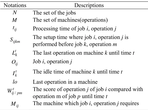
[image:3.595.47.293.101.299.2]The mathematical model was very useful since the value obtained after certain computation time can be used as a lower bound to evaluate the efficiency of the heuristic procedure. However, in larger problems, because of the combinatorial structure of the model finding optimum results is not reasonable. Hence, in this paper, three different lower bounds are developed which may be used to evaluate the heuristic models. Many researches such as [24], [25], [22], [26] developed different kind of lower bounds. These lower bounds would be useful to evaluate the performance of the heuristic models in larger problems. The following table describes the notations used in finding lower bounds and developing heuristic models.
Table 2: Notations Used in Lower Bounds and Heuristic Notations
Descriptions
N The set of the jobs
M The set of machines(operations)
ij
t
Processing time of job i, operation j
ijkm
S The setup time where job i, operation j is performed before job k, operation m t
k
L The last operation on machine k until time t ij
O Job i, operation j t
k
I The idle time of machine k until time t lo Last operation in a machine
t pm ij W /
The score of operation j of job i compared with
operation m of job p until time t ij
M
[image:3.595.299.553.601.790.2]The followings are three lower bound originated from the mentioned researches with some modifications:
⎪⎭ ⎪ ⎬ ⎫ + ⎩⎨ ⎧ =
∑
∑
− = + = ≠ = = = + )) ( min ( ) ( max 11 1... & ( 1) 1 ... 1 1 ) 1 ( M
j kmi j
M M i k N k M j ij N i S t LB j i km α (10) ⎭⎬ ⎫ + + ⎩ ⎨ ⎧ + + =
∑
=∑
∈ = − − = = Ni ij i N k N kjij
ij j i j i N i M j S t EF t ES LB
1 (1.. ) 1...
) 1 ( ) 1 ( ... 1 ... 1 2
' min( )
) ( ) ( min max (11) ⎩ ⎨ ⎧ ⎭⎬ ⎫ + + =
∑
∑
= ∈ = = Ni ij i N k N kjij
j M j S t L LB
1 (1.. ) 1... ...
1
3 max ( ) ' min ( ) (12)
{
1, 2, 3}
max LB LB LB
LB= (13) It should be mentioned that ESijandEFij, which are the
earlier start and finish time of operation j of job i, are
calculated as follows:
∑
− = = 1 1 j k ik ij tES (14)
∑
= + = M j k ik ij t EF1 (15) Note that LB1is job-based lower bound and LB2 and LB3 are machine-based lower bounds. Lkis the notation of each
machine which is originated from [26] which proved that the
n job m machine flow-shop minimum completion time
variance(CTV) problem reduces to a single machine CTV problem by considering the last operations of n jobs on
machine m. Nevertheless, the setup time could be
considered to determine the sequence of the last operations.
α is a binary variable which is equal to 1 if the setup times
should be performed in all machines in the presence of the jobs, otherwise it is equal to zero. LB1 calculates the minimum completion time of the jobs in non-delay conditions. LB2 is a machine base lower bound, which calculates the maximum completion time of all jobs in a machine. In this lower bound, for each machine, first, the sum of the processing time of all jobs which require that machine is calculated, and consequently the bound check if there is at least one operation that is in the first level of the sequence (first operation of a job). In other words, the earliest starting time of each machine is calculated and added to the sum of the processing times. This procedure is done as well for the operations that are in the last level of the sequence of their related jobs (last operations of the jobs). It is obvious that the total completion time is equal to at least one of the completion time of the jobs. Hence, if for any machine, there is not at least one operation, which is in the last level of the sequence of a job, the minimum remaining completion time of the jobs, is added to the lower bound. Note that '
) .. 1 ( N
i∈ means the sum of the (N-1)th
minimum setup times. In LB3, a new lower bound based on
the proposed lower bound in [26] is developed. For all lower bound the setup times is considered in order to have a good lower bound, which could be efficient in evaluating the models performance.
B. Definitions
In this section, we propose a new heuristic rule suitable for job shop scheduling with sequence dependent setup times. Scheduling procedures using dispatching rules are one of the effective methods available for job shop scheduling problems. The schedules rule using priority-dispatching rules in the forward scheduling approach are usually non-delay schedules. A non-non-delay schedule is one in which no machine is kept idle at any time when at least one job is waiting for processing. In this paper, a non-delay heuristic rule is developed based on the priority that each operation gains in each step. The major characteristic of these rules is the dynamic priority of operations during the steps of the procedure.
In this heuristic procedure whenever one or more machines become available at time t, the calculation process for all
available operations, which should process on available machines, is launched. Note that there may be more than one machine available at time t in the shop floor. In each
step of the procedure, an operation is selected if it follows all 3 conditions below:
Condition 1: All the predecessor of the operation should be
completed until time t.
Condition 2: The selected operation should have better
priority compared with all its competitors according to the mutual comparisons. According to this condition, at time t,
if there are n operations available following condition 1,
there may be n×(n−1)mutual comparisons. Note that a comparison is done where both operations require a same machine.
Condition 3: The setup times between the last operation on
the machine and the selected operation should be less than the idle time of that machine at time t. The idle time of
machine k at time t (Ikt) is the differences between the
current time and the last time where the machine became idle. Note that if all setup procedure performed in the presence of the jobs, the set up time could not be started until the related job is free from its previous operations. In both cases, if any operation passes only condition 1 and 2 but not condition 3, it can enter the operations waiting list. Whenever this operation passes condition 3, the model selects it to perform on its related machine.
C. Calculation the priority score:
Consider two operations j and m of jobs i and p that are
available at time t which both require machine k. The
priority score for both operations is calculated as follows:
) ( , max 1 1 / t k t k lopm M m z pz pm ij M j z iz t k loij ij t pm ij L lo I S t t t t I S T W ∈ ⎭ ⎬ ⎫ ⎥⎦ ⎤ ⎢⎣ ⎡ + + − ⎩ ⎨ ⎧ ⎢⎣ ⎡ ⎥⎦ ⎤ + − + =
∑
∑
+ = + + = (16)Finally, the operation with minimum W is selected. Note
the neighborhood search determines the best operation candidate to allocate to the machine k at time t.
Implementing condition 3 in various examples insures that
the quality of the final solution is affected by this condition. According to this condition, an operation, which won in mutual comparisons in previous step, should wait until its setup times between this operation and the last operation on the current machine is completed. Hence, although one selected operation has the best priority in the previous step, because of the new operations, which follow all conditions at the current time, it may have less priority than at least one of the new operations candidate for allocation to the machine. In order to show the performance of the proposed heuristic, a well-known example from the literature, which has four jobs and four machines, is selected [26]. The setup times are generated for each machine according to the a uniform discrete distribution U[0, min ti] which ti is the processing time of the tasks for each machine. It is assume that the setup times between operations in machine k could
not be greater than any processing time of operations, which require machine k. The following tables (Table 3 and Table
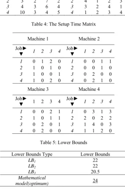
4) describe the example data. In Table 3, the processing times of operations and the machine sequencing for all jobs of the example are presented. Table 4 represents the setup times generated for all four machines.
The proposed algorithm seems to have good efficiency in large problems, which the mathematical solver could not find optimum solution in reasonable computational times. Implementing this heuristic insure that whenever a mutual comparison is implemented in the model, the algorithm makes better selection of operations. The ability of the proposed heuristic in finding feasible solutions in reasonable computational times which are near to the optimum solutions make it justifiable to use in job shop scheduling with sequence dependent setup times. The heuristic coded by Visual basic6, running by Pentium 4, CPU 2.4, with 256
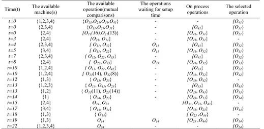
MB Ram, insures that proposed algorithm could reach on a feasible solution in a few seconds. In Table 5, all 3 lower bounds are calculated for the given example. Table 6 shows the final solution and Table (7) presents the main steps of the algorithm on the 4×4 example discussed in Table 3 and Table 4. As shown in Table 7, in many steps the mutual comparisons become necessary. It should be noted that where there are more than one operations available but they are belong to different machines, it is not essential to make the mutual comparisons and all the operations are selected directly and allocated to their specific machine. Nevertheless, in this algorithm, whenever an operation becomes available, if the setup times between this operation and the last operation on the related machine are less than the machine idle time, we consider the setup times in this idle times. It could be seen that for operations O24, O34, O43 and O44, the setup times begins before the times that their predecessors operations finish their process. The use of idle time of machine for setup consideration may results in better solution. The other specific feature of the heuristic is on the operations waiting for setup time. It should be mentioned that, although operations {O11, O33, O14} have both conditions 1 and 2, but the heuristic does not select them
deterministically until the setup time processing is finished. Note that it is assumed that setup time could be started even if the related job has not finished its operation in its previous level.
Table 3: Processing Time and Sequencing (Test Data) Processing Time Sequencing
Operations Operations
Job 1 2 3 4 Job 1 2 3 4
1 2 3 2 3 1 4 3 2 1
2 3 2 7 2 2 4 1 2 3
3 4 3 6 4 3 3 2 4 1
[image:5.595.299.550.185.563.2]4 10 3 4 5 4 1 2 3 4
Table 4: The Setup Time Matrix
Machine 1 Machine 2
Job►
▼ 1 2 3 4 Job▼► 1 2 3 4
1 0 1 2 0 1 0 0 1 1
2 1 0 1 0 2 0 0 1 0
3 1 0 0 1 3 0 2 0 0
4 1 0 2 0 4 0 2 1 0
Machine 3 Machine 4
Job►
▼ 1 2 3 4 Job▼► 1 2 3 4
1 0 0 2 1 1 0 3 1 3
2 1 0 1 1 2 2 0 2 2
3 0 2 0 1 3 1 4 0 3
4 0 2 0 0 4 1 1 2 0
Table 5: Lower Bounds Lower Bounds Type
Lower Bounds
LB1
22
LB2
22
LB3
20.5
Mathematical model(optimum)
[image:5.595.304.546.604.712.2]24
Table 6: The Test Data Sequencing (final solution)
Machines
Job 1 2 3 4
1 4 3 2 2
2 2 4 4 1
3 3 1 1 3
4 1 2 3 4
Completion
Table 7: Construction of the Schedule Using Proposed Heuristic
Time(t) The available machine(s) operation(mutual The available comparisons)
The operations waiting for setup
time
On process
operations The selected operation
t=0 {1,2,3,4} {O11,O21,O31,O41} - - {O41}
t=0 {2,3,4} {O11,O21,O31} - {O41} {O31}
t=0 {2,4} {O11(16),O21(13)} - {O41, O31} {O21}
t=3 {2,4} {O21, O11} - {O41, O31} -
t=4 {2,3,4} { O11, O32} O11 {O41} {O32}
t=5 {3,4} { O11, O22} O11 {O41, O32} {O11}
t=7 {2,3,4} { O12, O22, O33} - {O41} {O12}
t=8 {2,4} { O22, O33} O33 {O41, O12} {O33}
t=10 {1,2,4} { O13, O22, O42} - {O33} {O22}
t=10 {1,2,4} { O13(14), O42(8)} - {O33, O22} {O42}
t=12 {1,3} { O13, O23} - {O33, O42}
-t=13 {1,2,3} { O13, O43, O23} - {O33} {O43}
t=13 {1,2} { O13(11), O23(14)} - {O33, O43} {O13}
t=14 {1} { O34, O23} - {O43, O13} {O34}
t=15 {2,4} O14, O23 {O33, O23, O43} -
t=17 {3,4} { O14, O44} {O33, O23} {O44}
t=18 {1,3} { O14} { O23 ,O44}
-t=19 {1,3} O14 O14 {O23 ,O44} {O14}
t=22 {1,2,3,4} O24 - - {O24}
I. RESULTS
This paper addresses the job shop scheduling problem in the sequence-dependent setup time environment. Although, it is assumed that setup activity could be done on a machine even in the absence of any jobs on that machine, because of the flexibility of the both mathematical and heuristic models, the condition, which allows setup times to perform only in the presence of the jobs, could be easily considered in the model(α=1). In this paper, first a mathematical model, which is mixed-integer linear one, is developed. The mathematical model represents the good quality to find feasible solutions in reasonable computational time and weak quality to find optimum solutions. The combinatorial structure of the mathematical formulation insures that the efficient heuristic may have good solutions in reasonable computational times. Hence, a heuristics based on priority rules considering random generated setup times is developed. Implementing the heuristic in a problem found in the literature, which its optimum solution is definite, insures that the proposed heuristic have a good efficiency to reach a feasible solution equal to the optimum result. Nevertheless, three lower bounds are developed considering sequence dependent setup times, which will be useful to evaluate any heuristic, or meta-heuristic models performances in large problems which finding their optimum solution is not possible. Future researches may be on the performance of the heuristic to solve the various large problems, which their optimum result is not known. Hence, the lower bounds for solutions considering job-shop problems will be useful in future research. Metaheuristics such as Tabu Search, Simulated Annealing and Genetic algorithm are the other areas for future researches.
REFERENCES
[1] Ali Allahverdi a, C.T. Ng b, T.C.E. Cheng b, Mikhail Y. Kovalyov c, A survey of scheduling problems with setup times or costs, European Journal of Operational Research, 2006, doi:10.1016/j.ejor.2006.06.060
[2] Dessouky, M. M., & Leachman, R. C. Dynamic models of production with multiple operations and general processing times. Journal of the Operational Research Society, 1997, 48(6), pp.647–
654.
[3] Gomes, M. C., Barbosa-Povoa, A. P., & Novais, A. Q. Optimal scheduling for flexible job shop operation. International Journal of Production Research, 2005, 43(11), pp. 2323–2353
[4] Liu, M., Dong, M. Y., & Wu, C. An iterative layered tabu search algorithm for complex job shop scheduling problem. Chinese Journal of Electronics, 2005,14(3), pp.519–523.
[5] Liu, T. K., Tsai, J. T., & Chou, J. H. Improved genetic algorithm for the job-shop scheduling problem. International Journal of Advanced Manufacturing Technology, 2006,27(9–10), pp. 1021– 1029.
[6] Diaz-Santillan, E., & Malave, C. O. Simulated annealing for parallel machine scheduling with split jobs and sequence-dependent set-ups. International Journal of Industrial Engineering – Theory Applications and Practice, 2004, 11(1), pp. 43–53. [7] Blackstone, J. H., Philips, D. T., & Hogg, G. L. A state-of-the-art
survey of dispatching rules for manufacturingjob shopoperations. International Journal of Production Research, 1982,20, pp.27–45. [8] W.-H. Yang. Survey of scheduling research involving setup times.
Int. J Syst Sci ,1999;30.
[9] Allahverdi, A., Gupta, J.N.D., Aldowaisan, T, A review of scheduling research involving setup considerations. OMEGA The International Journal of Management Sciences,1999, 27, pp.219– 239]
[10] Zhou C, Egbelu PJ. Scheduling in a manufacturing shop with sequence-dependent setups. Robotics Computer Integrated Manufacturing ,1989;5: pp.73–81.
[11] Kim SC. Bowbrowski. impact of sequence dependent setup time on job shop scheduling performance. Int J Prod Res, 1994;32: pp.1503–20.
[13] .Focacci, F., Laborie, P., Nuijten, W., Solving scheduling problems with setup times and alternative resources. In:Proceedings of the Fifth International Conference on Artificial Intelligence Planning and Scheduling, Breckenbridge,Colorado, USA,2000, pp. 92–101. [14] .Choi I-C, Korkmaz O. Job shop scheduling with separable
sequencedependent setups. Ann Oper Res, 1997;70: pp.155–70. [15] .Ballicu, M., Giua, A., Seatzu, C.,. Job-shop scheduling models with set-up times. Proceedings of the IEEE International Conference on Systems, Man and Cybernetics, 2002,5, pp. 95– 100.
[16] Choi, I.C., Choi, D.S., A local search algorithm for jobshop scheduling problems with alternative operations and sequence-dependent setups. Computers and Industrial Engineering, 2002,2, pp. 43–58.
[17] Cheung, W., Zhou, H., Using genetic algorithms and heuristics for job shop scheduling with sequence-dependent setup times. Annals of Operations Research, 2001, 107, pp. 65–8.
[18] .Sun, J.U., Yee, S.R., Job shop scheduling with sequence dependent setup times to minimize makespan. International Journal of Industrial Engineering: Theory Applications and Practice, 2003, 10, pp.455–461.
[19] Garey MR, Johnson DS, Sethi R. The complexity of the flowshop and jobshop scheduling. Math Oper Res 1976;1: pp.117–29. [20] Hart, E., Ross, P., & Corne, D,Evolutionary scheduling: a review.
Genetic Programming and Evolvable Machines, 2005, 6, pp. 191– 220.
[21] Watanabe, M., Ida, K., & Gen, M. A genetic algorithm with modified crossover operator and search area adaptation for the jobshop scheduling problem. Computers and Industrial Engineering, 2005, 48(4), pp. 743–752.
[22] Zandieh, M., Fatemi Ghomi, S.M.T., Moattar Husseini, S.M., An immune algorithm approach to hybrid flow shopsscheduling with sequence-dependent setup times. Applied Mathematics and Computation, 2006, 180, pp.111–127.
[23] Lawrence, S., Resource Constrained Project Scheduling: An Experimental Investigation of Heuristic Scheduling Techniques (Supplement). Graduate School of Industrial Administration, Carnegie Mellon University, Pittsburgh, 1984.
[24] M.E. Kurz, R.G. Askin, Note on ‘‘an adaptable problem-space-based search method for flexible flow line scheduling’’, IIE Transactions , 2001 ,33 (8) pp. 691–693.
[25] M.E. Kurz, R.G. Askin, Scheduling flexible flow lines with sequence-dependent setup times, European Journal of Operational Research, 2004, 159 (1) , pp.66–82.