Alternative Analytical Method Used in Plotting the Shear Force and Bending Moment Diagrams, Translations and Rotations Distributions for Beams Subjected to Bending

Abstract - The actual graphical methods used by engineers

when plotting the stress distributions are based on integrating the differential equations of stresses for each beam segment. The resulting integration constants are obtained by imposing boundary conditions for each beam segment.

Using MATHCAD, this alternative proposed analytical method uses the step function Φ(x-a) which introduces a compact form of the stresses and displacements expressions. The constructive optimization is thus easier to be performed.

Index Terms – bending moment diagrams, foundations

I. INTRODUCTION

This article presents an alternate way of expressing the variation of the shear force Tz(x), bending moment Miy(x),

transversal cross-section rotations ϕy(x) and translations

w(x), using the MathCAD step function Φ(x-a), [1], [2], [3],

[4] having the well-known form:

⎩ ⎨ ⎧

≥ < =

− Φ

a x if

a x if a

x

1 0 )

( (1)

The practical application is the design of a continuous footing foundation placed under 4 columns. The axial compressive force in the columns is P. The layout of the

foundation is represented in fig.1 [5].

The properties of the soil under the footings leads to a loading model having as reactions the distributed loads q0

[5], [6].

For this loading model, the equilibrium condition between the exterior loads P and the reaction q0 will

become.

b a 3

P 4

q0= ₊ (2)

Manuscript received on October 17, 2007

C. M. is with Valahia University Targoviste ROMANIA, e-mail: marin_cor@yahoo.com,

V. F. is with Valahia University Targoviste ROMANIA, e-mail: v_filip@yahoo.com,

A. M. is a student of the Tehnical University of Constructions Bucharest ROMANIA e-mail: adu_de@yahoo.com

II. ANALYTICAL EXPRESSIONS

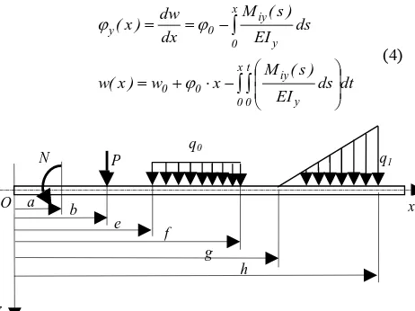
One considers a beam subjected to bending. The beam is characterized by length L and constant bending stiffness EIy.

There are 4 different load types, presented in fig. 2 [1], [2], [3], [4]:

- Bending moment N , at distance a from the left end of

the beam;

- Concentrated force P , at distance b from the left end of

the beam;

- Uniform distributed load q0 which acts on a beam

segment delimitated by the distances e and f from the

left end of the beam;

- Linear distributed load , x

[ ]

g,h g

h g x q ) x (

q ∈

− −

= ₁

which acts on a beam segment delimitated by the distances g and h from the left end of the beam.

The differential equation of translations w(x) and

rotations ϕy(x) corresponding to a cross-section is:

y iy

EI M

dx w

d ₌₋

2 2

(3)

Integrating twice the differential equation (2), one obtains after the first step, the rotations function ϕy(x).

Alternative Analytical Method Used in Plotting the

Shear Force and Bending Moment Diagrams,

Translations and Rotations Distributions for Beams

Subjected to Bending

[image:1.612.320.549.223.324.2]

Cornel Marin, Viviana Filip, Alexandru Marin

Fig 1.Continous footing loading scheme z

P P P P

b a a

a b

After the second integration the translations function w(x):

∫ ∫

∫

⎟ ⎟ ⎠ ⎞ ⎜ ⎜ ⎝ ⎛ − ⋅ + = − = = x 0 t 0 y iy 0 0 x 0 y iy 0 y dt ds EI ) s ( M x w ) x ( w ds EI ) s ( M dx dw ) x ( ϕ ϕ ϕ (4)

The analytical expressions of the shear force Tz(x),

bending moment Miy(x), transversal cross-section rotations ϕy(x) and translations w(x), for the loading types from fig. 2,

using the step function Φ are (EIy stiffness is constant):

For shear force:

(

)

(

)

(

)

₍

_{) (}

)

(

)

₍

_{) (}

x h

)

;

g h 2 ) h x ( q h x ) h x ( q g x g h 2 ) g x ( q f x ) f x ( q e x ) e x ( q b x P ) x ( T 2 1 1 2 1 0 0 z − ⋅ − − ⋅ + − ⋅ − ⋅ + + − ⋅ − − ⋅ − − ⋅ − ⋅ + + − ⋅ − ⋅ − − ⋅ − = Φ Φ Φ Φ Φ Φ (5)

For bending moment:

(

)

(

) (

)

(

)

(

)

(

) (

)

(

)

(

) (

x h

)

; g h 6 ) h x ( q h x 2 ) h x ( q g x g h 6 ) g x ( q f x 2 ) f x ( q e x 2 ) e x ( q b x b x P a x N ) x ( M 3 1 2 1 3 1 2 0 2 0 iy − ⋅ − − ⋅ + + − ⋅ − ⋅ + − ⋅ − − ⋅ − − − ⋅ − ⋅ + − ⋅ − ⋅ − − − ⋅ − ⋅ − − ⋅ − = Φ Φ Φ Φ Φ Φ Φ (6)

For the cross-sectional rotations functions

(

) (

)

(

)

₍

₎

₍

₎

(

)

₍

_{) (}

)

(

)

₍

_{) (}

x h

)

;

g h 24 ) h x ( q h x 6 ) h x ( q g x g h 24 ) g x ( q f x 6 ) f x ( q e x 6 ) e x ( q b x 2 b x P a x a x N EI ) x ( EI 4 1 3 1 4 1 3 0 3 0 2 0 y y y − ⋅ − − ⋅ − − ⋅ − ⋅ − − − ⋅ − − ⋅ + − ⋅ − ⋅ − − − ⋅ − ⋅ + − ⋅ − ⋅ + + − ⋅ − ⋅ + = Φ Φ Φ Φ Φ Φ Φ ϕ ϕ (7)

For the cross-sectional displacements functions

(

)

₍

₎

(

)

₍

₎

₍

₎

(

)

₍

_{) (}

)

(

)

₍

_{) (}

x h

)

;

g h 120 ) h x ( q h x 24 ) h x ( q g x g h 120 ) g x ( q f x 24 ) f x ( q e x 24 ) e x ( q b x 6 b x P a x 2 a x N x EI w EI ) x ( w EI 5 1 4 1 5 1 4 0 4 0 3 2 0 y 0 y y − ⋅ − − ⋅ − − ⋅ − ⋅ − − − ⋅ − − ⋅ + − ⋅ − ⋅ − − − ⋅ − ⋅ + − ⋅ − ⋅ + + − ⋅ − ⋅ + ⋅ + = Φ Φ Φ Φ Φ Φ Φ ϕ (8)

III. APPLICATION OF COMPUTING FOUNDATION DIAGRAMS

The application’s task is to obtain the required diagrams for the continuous footing foundation represented by the model in fig. 1 using the step function. The required diagrams will be:

- shear force diagrams Tz(x);

- bending moment diagrams Miy(x);

- cross-sectional rotations distribution ϕy(x)

- cross-sectional displacements distribution w(x)

(settlements of the soil under the foundation),

Considering the symmetry of the system from fig. 1, the following analytical expressions will be written using the step function:

x∈(0; b+1.5a)

shear force:

(

)

(

)

(

)

( )

(

)

(

x b

)

;

b 2 ) b x ( q b x ) b x ( q x b 2 x q b x ) b x ( q b a x P b x P ) x ( T 2 1 1 2 1 0 z − ⋅ − ⋅ − − ⋅ − ⋅ − − ⋅ ⋅ + − ⋅ − ⋅ + + − − ⋅ − − ⋅ − = Φ Φ Φ Φ Φ Φ (9) bending moment:

(

) (

)

(

) (

)

(

)

( )

(

)

(

x b

)

;

b 6 ) b x ( q b x 2 ) b x ( q x b 6 x q b x 2 ) b x ( q b a x b a x P b x b x P ) x ( M 3 1 2 1 3 1 2 0 iy − ⋅ − ⋅ − − ⋅ − ⋅ − − ⋅ ⋅ + − ⋅ − ⋅ + + − − ⋅ − − ⋅ − − − ⋅ − ⋅ − = Φ Φ Φ Φ Φ Φ (10) cross-sectional rotation:

(

)

(

)

(

)

( )

x

[image:2.612.75.306.65.238.2]

b 24 x q b x 6 ) b x ( q b a x 2 ) b a x ( P b x 2 ) b x ( P EI ) x ( EI 4 0 3 0 2 2 0 y y y + ⋅ ⋅ − − ⋅ − ⋅ − − − − ⋅ − − ⋅ + + − ⋅ − ⋅ + = Φ Φ Φ Φ ϕ ϕ (11) Fig 2. Beam model loaded with 4 different loading

z

O a _{b x}

cross-sectional displacement:

(

)

(

)

(

)

( )

(

)

(

x b

)

b 120 ) b x ( q b x 24 ) b x ( q x b 120 x q b x 24 ) b x ( q b a x 6 ) b a x ( P b x 6 ) b x ( P x EI w EI ) x ( w EI 5 0 4 0 5 0 4 0 3 3 0 y 0 y y − ⋅ − ⋅ + − ⋅ − ⋅ + + ⋅ ⋅ − − ⋅ − ⋅ − − − − ⋅ − − ⋅ + + − ⋅ − ⋅ + ⋅ + = Φ Φ Φ Φ Φ Φ ϕ (12)

The initial parameters will be determined using the following conditions:

- the settlement under the columns depends on the pressure distribution q0 and the corresponding tributary area [4]:

(

P q a

)

c ) a b ( w 2 b a q P c ) b ( w 0 0 ⋅ − ⋅ = + ⎟ ⎠ ⎞ ⎜ ⎝ ⎛ _{− ⋅} + ⋅ = (13)

- the rotation of the middle section of the beam is null:

0 ) a 5 . 1 b (

y + =

ϕ (14)

Denoting in (11) relation:

(

)

(

)

(

)

( )

(

)

(

x b

)

;

b 24 ) b x ( q b x 6 ) b x ( q x b 24 x q b x 6 ) b x ( q b a x 2 ) b a x ( P b x 2 ) b x ( P ) x ( F 4 0 3 0 4 0 3 0 2 2 − ⋅ − ⋅ + − ⋅ − ⋅ + + ⋅ ⋅ − − ⋅ − ⋅ − − − − ⋅ − − ⋅ + + − ⋅ − ⋅ = Φ Φ Φ Φ Φ Φ (15)

and in (12) relation:

(

)

(

)

(

)

( )

(

)

(

x b

)

b 120 ) b x ( q b x 24 ) b x ( q x b 120 x q b x 24 ) b x ( q b a x 6 ) b a x ( P b x 6 ) b x ( P ) x ( W 5 0 4 0 5 0 4 0 3 3 − ⋅ − ⋅ + − ⋅ − ⋅ + + ⋅ ⋅ − − ⋅ − ⋅ − − − − ⋅ − − ⋅ + + − ⋅ − ⋅ = Φ Φ Φ Φ Φ Φ (16)

Introducing the conditions (13) and (14), the constant c

and the initial parameters ϕ0and w0 are obtained:

(

P q a

)

c ) a b ( W ) a b ( EI w EI ) a 5 . 1 b ( F EI ) b ( W ) a b ( W a EI 2 a b q c 0 0 y 0 y 0 y 0 y 0 ⋅ − ⋅ + + − + ⋅ − = + − = − + + ⋅ = − ⋅ ⋅ ϕ ϕ ϕ (17)

IV. NUMERICAL APPLICATION

The above mentioned relations will be used, for three numerical values hypotheses of the current application.

Hypothesis 1

Replacing in MathCAD the parameters values: P=10kN;

b=1m; a=3 m; EI=106 N⋅m2 the variation diagrams for half

of the foundation are obtained (fig. 3 , fig.4 and fig.5.)

0 0.5 1 1.5 2 2.5 3 3.5 4 4.5 5 5.5

1

− ×104 6

− ×103 2

− ×103 2 10× 3

6 10× 3

1 10× 4

M x( )

−

Axa x( )

T x( )

[image:3.612.73.298.79.191.2]

x

Fig 3. Shear force and bending moment diagrams

0 0.5 1 1.5 2 2.5 3 3.5 4 4.5 5 5.5

0.04 − 0.032 − 0.024 − 0.016 − 8 − ×10−3

0

f x( ) Axa x( )

[image:3.612.316.530.196.333.2]

x

Fig 4. Cross-sectional rotations distribution

0 0.5 1 1.5 2 2.5 3 3.5 4 4.5 5 5.5

0.1 − 0.05 − 0 0.05 0.1

w x( )

Axa x( )

x

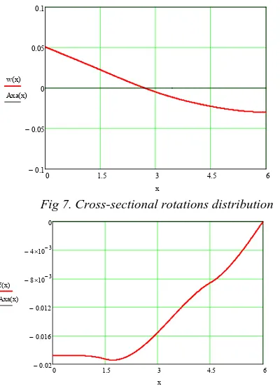
[image:3.612.65.525.280.676.2] [image:3.612.73.295.335.589.2]

Hypothesis 2

Replacing in MathCAD the parameters values: P=10kN;

b=1.5m; a=3 m; EI=106 N⋅m2 the variation diagrams for

half of the foundation are obtained (fig. 6 , fig.7 and fig.8)

Hypothesis 3

Replacing in MathCAD the parameters values: P=10kN;

b=2m; a=3 m; EI=106 N⋅m2 the variation diagrams for half

of the foundation are obtained (fig. 9, fig. 19 and fig. 11).

V. CONCLUSIONS

- This is an method of expressing the variation of the shear force Tz(x), bending moment Miy(x), transversal

cross-section rotations ϕy(x) and translations w(x),

using the MathCAD step function Φ(x-a) in a more

compact way than the traditional methods.

- This method is well suited for the constructive

optimization of the structure, using the obtained numerical values and varying different parameters: in the current application, the length of the cantilever b

was changed for optimization purposes.

- Analyzing the 3 sets of diagrams, it’s obvious that the

best bending moment distribution and the best displacements case will correspond to the largest value of the cantilever length b. (3rd Hypothesis).

- Considering the fact that the step function method uses

simple operation expressions, the numerical applications are being solved fast with a minimum number of computational cycles. The traditional methods use integral expressions which are solved by means of numerical methods. These methods imply a large number of computational cycles, which will cause slower obtained results.

0 1.5 3 4.5 6

1 − ×104

6 − ×103

2 − ×103

2 10× 3 6 10× 3 1 10× 4

M x( ) − Axa x( ) T x( )

[image:4.612.317.529.66.406.2]

x

Fig 6. Shear force and bending moment diagrams

0 1.5 3 4.5 6

0.1

−

0.05

−

0 0.05 0.1

w x( )

Axa x( )

x

Fig 7. Cross-sectional rotations distribution

0 1.5 3 4.5 6

0.02 −

0.016 −

0.012 − 8 − ×10−3

4 − ×10−3

0

f x( ) Axa x( )

x

Fig 8. Cross-sectional displacements distribution

0 0.5 1 1.5 2 2.5 3 3.5 4 4.5 5 5.5 6 6.5

0.1

−

0.05

−

0 0.05 0.1

w x( )

Axa x( )

x

Fig 11. Cross-sectional displacements distribution

2 − ×103

2 10× 3 6 10× 3 1 10× 4

M x( ) − Axa x( ) T x( )

0 0.5 1 1.5 2 2.5 3 3.5 4 4.5 5 5.5 6 6.5

0.02

−

0.016

−

0.012

−

8

− ×10−3 4

− ×10−3 0

f x( )

Axa x( )

[image:4.612.78.279.101.224.2]

x

[image:4.612.85.285.254.530.2] [image:4.612.74.280.612.734.2]

VI. REFERENCES

[1] C. Marin, ”Rezistenţa materialelor şi elemente de teoria elasticităţii”. Editura Biblioteca, 2006,

http://fsim.valahia.ro/cursuri.html

[2] C. Marin, ”Aplicaţii ale teoriei elasticităţii în inginerie”. Editura Biblioteca, 2007, http://fsim.valahia.ro/cursuri.html

[3] C. Marin, A. Marin, ”Metoda analitica pentru trasarea diagramelor de eforturi în barele drepte”. SIMEC 2006, UTCB Bucuresti , 2006, pp.81-86

[4] C. Marin, A. Marin, ”Metoda analitica pentru calculul deplasărilor şi rotirilor barelor drepte supuse la încovoiere”, SIMEC 2006, UTCB Bucuresti , 2006, pp.87-92

[5] I. Manoliu, ”Geotehnicăşi fundaţii”, Editura Tehnică

Bucureşti, 1986.