A. Binary Particle Swarm Optimization

Abstract_{—Feature selection is a useful technique for} increasing classification accuracy. The primary objective is to remove irrelevant features in the feature space and identify relevant features. Binary particle swarm optimization (BPSO) has been applied successfully in solving feature selection problem. In this paper, chaotic binary particle swarm optimization (CBPSO) with logistic map for determining the inertia weight is used. The K-nearest neighbor (K-NN) method with leave-one-out cross-validation (LOOCV) serves as a classifier for evaluating classification accuracies. Experimental results indicate that the proposed method not only reduces the number of features, but also achieves higher classification accuracy than other methods.

Index Terms—Feature selection, binary particle swarm optimization, logistic map, K-nearest neighbor, leave-one-out cross-validation.

I. INTRODUCTION

Feature selection is the process of choosing a subset of features from the original feature set and thus can be viewed as a principal pre-processing tool prior to solving classification problems [1]. Feature selection is a NP-hard problem. The goal is to select a subset of d features from a set of D features (d < D) in a given data set [2]. D is comprised of all features in a given data set; it may include noisy, redundant, and misleading features. Therefore, an exhaustive search performed in the solution space, which usually takes a long time, often does not work in practice [3]. To resolve these feature selection problems, we aimed at retaining only d relevant features. Irrelevant features are not only useless for classification, but could also potentially reduce the classification performance. By deleting irrelevant features computational efficiency can be improved and classification accuracy increased.

Three different categories of evaluation criteria can be employed when deciding which features are relevant and which ones should be removed: filters, wrapper and hybrid models [4]. The filter model relies on general characteristics

Manuscript received January 4, 2008. (Li-Yeh Chuang is with the Department of Chemical Engineering, I-Shou University, Kaohsiung, Taiwan (email: [email protected]))

Jung-Chike Li is with the Department of Electronic Engineering, National Kaohsiung University of Applied Sciences, Taiwan (e-mail: [email protected]).

Cheng-Hong Yang is with the Department of Electronic Engineering, National Kaohsiung University of Applied Sciences, Taiwan (e-mail: [email protected])

of the data to evaluate and select feature subsets without involving any learning algorithm [4]. Wrapper models apply an unsupervised learning algorithm to each subset of features and then evaluate the subset of features by criterion functions [5]. Wrapper models usually have a higher computational cost than the filter modes. Hybrid models attempt to take advantage of the two models by exploiting their different evaluation criteria at different search stages, and have recently been proposed to handle large data sets [4].

We adopted a wrapper model to work on the feature selection problem. In recent years, different evolutionary algorithms have been proposed to obtain near-optimal subsets of solutions. These approaches include genetic algorithms (GA) designed by imitating natural evolution [2], ant colony optimization (ACO)[6], particle swarm optimization (PSO) [1]with swarm intelligence and tabu search (TS) [7] with intermediate memory.

Particle swarm optimization is a search process based on the idea of swarm intelligence in biological populations. In PSO, an information sharing algorithm randomly generates an initial population for the search process. The position and velocity of each particle is adjusted based on its individual experience and the experience of its neighbors. The information is updated due to social interactions between particles.

In this paper, chaotic binary particle swarm optimization (CBPSO) with logistic map for determining the inertia weight is used. The K-nearest neighbor (K-NN) method based on Euclidean distance calculations serves as a classifier for five data sets taken from the literature [2]. Experimental results show that CBPSO can not only reduce the number of features, but also achieves higher classification accuracies.

II.METHOD

A. Binary Particle Swarm Optimization

Particle Swarm Optimization (PSO) is a population-based evolutionary computation technique developed by Kennedy and Eberhart in 1995 [8]. PSO simulates the social behavior of animals, i.e. birds in a flock or fish in a school. This behavior can be described by a swarm intelligence system. In PSO, each solution can be considered an individual particle in a given search space, which has its own position and velocity. During movement, each particle adjusts its position by changing its velocity based on its own experience, as well as the experience of its neighboring particles, until an optimum position is reached by itself and its neighbor [9]. All of the particles have fitness values based on the calculation of a

Chaotic Binary Particle Swarm Optimization

for Feature Selection using Logistic Map

fitness function. Particles are updated by following two parameters called pbest and gbest at each iteration. Each particle is associated with the best solution (fitness) the particle has achieved so far in the search space. This fitness value is stored, and represents the position called pbest. The value gbest is a global optimum value for the entire population.

PSO was originally developed to solve real-value optimization problems. Many optimization problems occur in a space featuring discrete, qualitative distinctions between variables and levels of variables. To extend the real-value version of PSO to a binary/discrete space, Kennedy and Eberhart proposed a binary PSO (BPSO) method. In a binary search space, a particle may move to near corners of a hypercube by flipping various numbers of bits; thus, the overall particle velocity may be described by the number of bits changed per iteration [10].

The position of each particle is represented by Xp = {Xp1, Xp2, …, Xpd} and the position of each particle is represented in binary string form and is randomly generated; the bit value {0} and {1} represent a non-selected and selected feature, respectively. The velocity of each particle is represented by Vp = {Vp1, Vp2, …, Vpd} (d is number of particles) and the initial velocities in particles are probability limited to a range of {0.0~1.0}. In BPSO, once the adaptive values pbest and gbest are obtained, the features of the pbest and gbest particles can be tracked with regard to their position and velocity. Each particle is updated according to the following equations [10].

(

)

(

)

pd d old pd pd old pd new

pd w v c rand pbest x c rand gbest x

v = × +₁× ₁× − +₂× ₂× − (1)

if vnewpd ∉(Vmin, Vmax) then

new pd

v = max (min (Vmax,vnewpd ), Vmin) (2)

(

)

pd v new pd e v S − + = 1 1 (3) (3)

If

(

(

)

)

In Eq.(1), w is the inertia weight, c1 and c2 are acceleration parameters, and rand, rand1 and rand2are three

independent random numbers between [0, 1]. Velocities new pd

v

and old pd

v are those of the updated particle and the particle before being updated, respectively, old

pd

x is the original particle position (solution), and new

pd

x is the updated particle position (solution). In Eq. (2), particle velocities of each dimension are tried to a maximum velocityV_max. If the sum of accelerations causes the velocity of that dimension to exceedV_max, then the velocity of that dimension is limited toV_max. Vmax and Vminare user-specified parameters (in our case V_max= 6, Vmin= -6). The updated features are calculated by the function S(vnewpd ) (Eq. (3)), in which

new pd

v is the updated velocity value. If S(vnewpd ) is larger than a randomly produced

disorder number that is within {0.0~1.0}, then its position value Sn, n=1, 2, K, m is represented by {1} (meaning this feature is selected as a required feature for the next

update). If S(vnewpd ) is smaller than a randomly produced

disorder number that is within {0.0~1.0}, then its position value Fn, n=1, 2, K, m is represented by {0} (meaning this feature is not selected as a required feature for the next update).

Two independent numbers, rand₁and rand2in Eq. (1), affect the velocity of each particle. The proper adjustment of the BPSO parameters w (inertia weight) and the acceleration factors c₁ and c₂ is an important task. The inertia weight wcontrols the balance between the global exploration and local search ability. c₁ and c₂control the movement of particles. To avoid premature BPSO convergence, the adjustment can not be too excessive, since this might cause extreme particle movements, which it makes impossible to obtain optimized features. Hence, suitable parameter adjustment is paramount.

B.Chaotic Sequences for Inertia Weight

The inertia weight wcontrols the balance between the global exploration and local search ability. A large inertia weight facilitates the global search, while a small inertia weight facilitates the local search. How to adjust the inertia weight value is important; it will affect the BPSO search process and through it the classification accuracy.

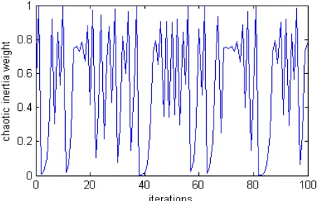
The BPSO process suffers from getting trapped in a local optimum which results in premature convergence. In order to prevent this from happening, we used chaotic binary particle swarm optimization to overcome the disadvantage. Chaos is a deterministic dynamic system and is very sensitive to initial values. A chaotic map is used to determine the inertia weight value in each iteration. Logistic map is the most frequently used chaotic behavior and is a bounded unstable dynamic behavior. In this paper, we used logistic map to determine the inertia weight value [11]. The inertia weight value is modified according to

w (t + 1) = 4.0 × w(t) × (1 – w(t)) w(t) ∈(0,1) (5) The inertia weight value depends on the chaotic logistic map for total iterations shown in Figure 1

Figure 1 Chaotic inertia weight using logistic map

C.K-Nearest Neighbor

learning algorithm introduced by Fix and Hodges in 1951, and is still one of the most popular nonparametric methods [12][13]. The K-NN method is easy to implement since only the parameter K (number of nearest neighbors) needs to be determined. The parameter K is the most important factor affecting the performance of the classification process. In a multidimensional feature space, the data is divided into testing and training samples. K-NN classifies a new object based on the minimum distance from the test samples to the training samples based either their Euclidean or Mahalanobis distance. We used the Euclidean distance in this paper. If an object is near to the number of K nearest neighbors, the object is classified into the K-object category. In order to increase the classification accuracies, the parameter K has to be adjusted based on the different data set characteristics.

In K-NN, a large category tends to have a small classification error, while the classification error for minority classes is usually rather large, a fact that lowers the performance of K-NN [14]. Cross-validation is a useful technique for choosing the parameter K. In this paper, the leave-one-out cross-validation (LOOCV) method was implemented. When there aren data to be classified, the data is divided into one testing sample and n-1 training samples at each iteration of the evaluation process, and finally a classifier is constructed by training the n-1 training samples. The testing sample category can be judged by the classifier. In this paper, the 1-NN with leave-one-out cross-validation method serves as a classifier to calculate the classification accuracies.

D.CBPSO -KNN procedure

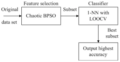
Initially, the position of each particle is represented by a binary (0/1) stringS=F1F2LFD. D is the dimension of a given data set where 1 represents a selected feature, while 0 represents a non-selected feature. For example, for D=10, we obtain a random binary string S=1000100010, which means that only features F1, F5 and F9 are selected. The initial velocities in particles are probability limited to a range of {0.0~1.0}.Figure 2 shows the three stages employed in this study.

Figure 2 Simple three stages for feature selection

The classification accuracy of a 1-nearest neighbor (1-NN) determined by the leave-one-out cross-validation method is used to measure the fitness of each particles. CBPSO procedure can be described as follows:

Step 1 Randomly generate an initial population for CBPSO. Step 2 Evaluate fitness values of all particles.

Step 3 Update the pbest and gbest values. Each particle

updates its position and velocity by CBPSO through updates Eqs. (1) (2) (3) (4) (5).

Step 4 Check the termination criterion. If satisfied, output final solution. Otherwise go to Step 2.

The CBPSO was configured to contain 20 particles which the number of particles is equal to the populations of HGAs from the literature.The termination criterion is 100 iterations. The acceleration factors c1 and c2 were both set to 2 [15]. The inertia weight w(0) was 0.48 [11]

III. RESULTS AND DISCUSSION

The data sets in this study were obtained from the UCI Repository [16]. Table 1 illustrates the format of the five classification problems. Three different feature selection problems were classified. If the number of features is between 10 and 19, the sample groups can be considered small; these data sets included the Wine, Vehicle and Segmentation data sets. If the number of features is between 20 and 49, the sample test groups are medium scale problems; these include the WDBC problems. If the number of features is greater than 50, the test problems are large scale problems; this group included the Sonar problem. The classifier used was the 1-NN method with leave-one-out cross-validation for all five data sets.

Table 1 Format of classification test problems

Data sets Number of samples

Number of classes

Number of features

Wine 178 3 13

Vehicle 846 4 18

Segmentation 210/2100 7 19

WDBC 569 2 30

Sonar 208 2 60

Legend: x/y indicates the number of testing and training samples, respectively

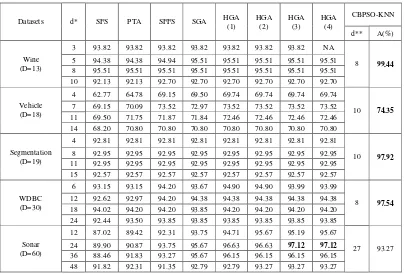
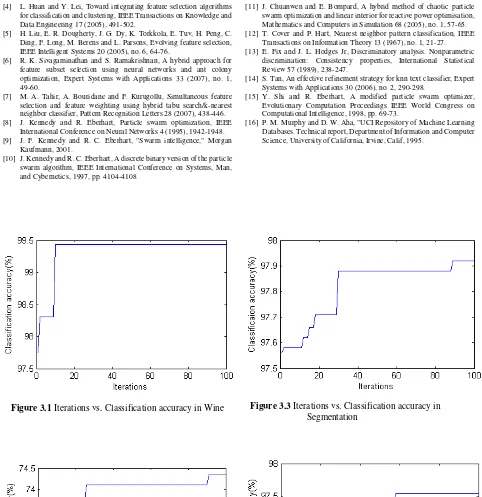
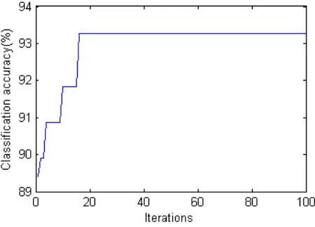
Table 2 compares experimental results obtained by other methods from the literature [2] to the proposed method. The proposed method obtained the highest classification accuracy for the Wine, Vehicle, Segmentation and WDBC classification problems. The classification accuracies of the Wine, Vehicle, WDBC and Segmentation classification problems obtained by the proposed method are 99.44%, 74.35%, 97.54% and 97.92%, respectively. The proposed method obtained a lower classification accuracy for the Sonar classification problem. The classification accuracy for the Sonar classification problem obtained by the proposed method is 93.27%. Figures 3.1-3.5 show the Iterations vs. Classification accuracy for five test data sets.

Table 3 Classification accuracies for the test data sets

Legend: D: total number of features, d*: selected number of features, SFS: sequential forward search, PTA: plus and take away, SFFS: sequential forward floating search, SGA: sequential Genetic Algorithm, HGA: hybrid Genetic Algorithm, d**: optimal selected number of features, CBPSO-KNN: Chaotic BPSO with K-NN, A(%): classification accuracy in %, Highest values are in bold-type.

literature, obtained lower classification accuracies, a fact clearly illustrated by the Wine test problem, for which the classification accuracy obtained by the proposed method was higher than the results from the literature, while the number of features selected was the same. From Table 3, GA has been shown to outperform SFS (sequential forward search), PTA (plus and take away) and SFFS (sequential forward floating search) from the literature [2]. In this study, we used three differently sized categories of test problems, namely small, medium and large size problems. If the feature dimensionality is between 10 and 19, the sample groups can be considered small size problems. If the feature dimensionality is between 20 and 49, the sample group test problems are of medium size problems. If the feature dimensionality is over 50, the test problems are large size problems. Results in Table 2 indicate that, CBPSO works well for small and medium size problems, although for high-dimension problems, like the Sonar test problem, CBPSO may become trapped in a local optimal region. Overall, CBPSO has competitive performance in feature selection problems.

A chaos system has certain, ergodic and stochastic properties. Using chaotic behavior in the inertia weight value with logistic map would cause the inertia weight values to fluctuate between [0, 1]. The changed inertia weight values affect the velocities and positions of particles at each iteration. Introducing a fluctuating inertia weight value, the particles to move on to new search regions. Extending the search space region is an important task. Chaotic behavior increases the local and global search ability. A group of particles may search new regions of the solution space and congregate

toward a global or near-global optimum. This extended search in the solution space is equivalent to different subset combinations of features which lead to superior classification.

IV. CONCLUSION

In recent years, different evolutionary algorithms have been developed for feature selection. In this paper, a new feature selection method based on chaotic binary particle swarm optimization (CBPSO) is proposed. The classification accuracy is calculated by a 1-NN classifier with LOOCV. The proposed method saves computing time compared to other methods from the literature. CBPSO with chaotic sequences for the inertia weight is applied to feature selection process. Experimental results indicate that the proposed method not only effectively reduces the number of features, but also achieves higher classification accuracy. CBPSO is very competitive compared to other methods and can serve as an ideal pre-processing tool to help optimize the feature selection process.

REFERENCES

[1] X. Wang, J. Yang, X. Teng, W. Xia and R. Jensen, Feature selection based on rough sets and particle swarm optimization, Pattern Recognition Letters 28 (2007), no. 4, 459-471.

[2] I.-S. Oh, J.-S. Lee and B.-R. Moon, Hybrid genetic algorithms for feature selection, IEEE Transactions on Pattern Analysis and Machine Intelligence 26 (2004), 1424-1437.

[3] T. M. Cover and J. M. Van Campenhout, On the possible orderings in the measurement selection problem, IEEE Trans. Systems, Man, and Cybernetics 7 (1977), no. 9, 657-661.

Datasets d* SFS PTA SFFS SGA HGA

(1)

HGA (2)

HGA (3)

HGA (4)

CBPSO-KNN

d** A(%)

Wine (D=13)

3 93.82 93.82 93.82 93.82 93.82 93.82 93.82 NA

8 99.44

5 94.38 94.38 94.94 95.51 95.51 95.51 95.51 95.51 8 95.51 95.51 95.51 95.51 95.51 95.51 95.51 95.51

10 92.13 92.13 92.70 92.70 92.70 92.70 92.70 92.70

Vehicle (D=18)

4 62.77 64.78 69.15 69.50 69.74 69.74 69.74 69.74

10 74.35

7 69.15 70.09 73.52 72.97 73.52 73.52 73.52 73.52 11 69.50 71.75 71.87 71.84 72.46 72.46 72.46 72.46 14 68.20 70.80 70.80 70.80 70.80 70.80 70.80 70.80

Segmentation (D=19)

4 92.81 92.81 92.81 92.81 92.81 92.81 92.81 92.81

10 97.92

8 92.95 92.95 92.95 92.95 92.95 92.95 92.95 92.95

11 92.95 92.95 92.95 92.95 92.95 92.95 92.95 92.95 15 92.57 92.57 92.57 92.57 92.57 92.57 92.57 92.57

WDBC (D=30)

6 93.15 93.15 94.20 93.67 94.90 94.90 93.99 93.99

8 97.54

12 92.62 92.97 94.20 94.38 94.38 94.38 94.38 94.38 18 94.02 94.20 94.20 93.85 94.20 94.20 94.20 94.20 24 92.44 93.50 93.85 93.85 93.85 93.85 93.85 93.85

Sonar (D=60)

12 87.02 89.42 92.31 93.75 94.71 95.67 95.19 95.67

27 93.27 24 89.90 90.87 93.75 95.67 96.63 96.63 97.12 97.12

[4] L. Huan and Y. Lei, Toward integrating feature selection algorithms for classification and clustering, IEEE Transactions on Knowledge and Data Engineering 17 (2005), 491-502.

[5] H. Liu, E. R. Dougherty, J. G. Dy, K. Torkkola, E. Tuv, H. Peng, C. Ding, F. Long, M. Berens and L. Parsons, Evolving feature selection, IEEE Intelligent Systems 20 (2005), no. 6, 64-76.

[6] R. K. Sivagaminathan and S. Ramakrishnan, A hybrid approach for feature subset selection using neural networks and ant colony optimization, Expert Systems with Applications 33 (2007), no. 1, 49-60.

[7] M. A. Tahir, A. Bouridane and F. Kurugollu, Simultaneous feature selection and feature weighting using hybrid tabu search/k-nearest neighbor classifier, Pattern Recognition Letters 28 (2007), 438-446. [8] J. Kennedy and R. Eberhart, Particle swarm optimization, IEEE

International Conference on Neural Networks 4 (1995), 1942-1948. [9] J. F. Kennedy and R. C. Eberhart, "Swarm intelligence," Morgan

Kaufmann, 2001.

[10] J. Kennedy and R. C. Eberhart, A discrete binary version of the particle swarm algorithm, IEEE International Conference on Systems, Man, and Cybernetics, 1997, pp. 4104-4108

Figure 3.1 Iterations vs. Classification accuracy in Wine

Figure 3.2 Iterations vs. Classification accuracy in Vehicle

[11] J. Chuanwen and E. Bompard, A hybrid method of chaotic particle swarm optimization and linear interior for reactive power optimisation, Mathematics and Computers in Simulation 68 (2005), no. 1, 57-65. [12] T. Cover and P. Hart, Nearest neighbor pattern classification, IEEE

Transactions on Information Theory 13 (1967), no. 1, 21-27. [13] E. Fix and J. L. Hodges Jr, Discriminatory analysis. Nonparametric

discrimination: Consistency properties, International Statistical Review 57 (1989), 238-247.

[14] S. Tan, An effective refinement strategy for knn text classifier, Expert Systems with Applications 30 (2006), no. 2, 290-298.

[15] Y. Shi and R. Eberhart, A modified particle swarm optimizer, Evolutionary Computation Proceedings IEEE World Congress on Computational Intelligence, 1998, pp. 69-73.

[16] P. M. Murphy and D. W. Aha, "UCI Repository of Machine Learning Databases. Technical report, Department of Information and Computer Science, University of California, Irvine, Calif, 1995.

Figure 3.3 Iterations vs. Classification accuracy in Segmentation