Abstract—For the analysis and forecasting of time series, we always search for a statistical model capable of understanding the underlying processes of data and filtering the unwanted noise. This noise may either be white or coloured, having some pattern of autoregressive moving average i.e., ARMA(p,q) processes. This search is carried out by using various forecast accuracy criteria and tools such as, Akaike’s information criterion (AIC) and Akram test statistic (ATS).
As compared to others, the AIC and ATS are noted to be more effective for identification of good models. However, AIC, being parametric in nature, is found to be comparatively more sensitive to noise volatilities and cumbersome to use; whereas, ATS, the base of which is distribution free is observed to be quite robust to noise variations, parsimonious in nature and relatively more easy to use. In this paper both the AIC and ATS are reviewed, practical implication discussed and their role in identifying optimum models from a class of candidate statistical models, especially, the linear dynamic system models is examined. For better insight, into these gadgets an example on analysis and forecasting of daily copper prices is given.
Index Terms—Akaike’s information criterion, Akram test statistic, optimum forecast, statistical models, ASL, Coloured noise.
1 Introduction
Model selection is a decision theoretic approach. The main purpose is to identify the model that shows the best balance between data fitting and model complexity. Information criteria offer various procedures to choose the best model amongst a set of many possible models through certain guiding principles in particular situations but not across a variety of situations. Akaike [1] found the unbiased estimator of (relative) Kullback-Leibler (K-L) information or distance which is simply the distance between the true density and estimated density for each model.
Prof. Akram M. Chaudhry is with the College of Business Administration, University of Bahrain, Sakhir, Kingdom of Bahrain, Middle East.
Tel. +973 39171071 (e-mail: [email protected])
Irfan Ahmed is working for PhD (Statistics) in the area of dynamic forecasting modelling at the University of Lahore, Lahore, Pakistan under the supervision of Prof. Akram M. Chaudhry. He is Deputy Manager, Warehouse & Inventory Management with Pakistan Water and Power Development Authority at Faisalabad, Pakistan. (e-mail: [email protected])
The basic objective of this paper is not only to explain and compare Akaike’s information criterion (AIC) and Akram test statistic (ATS), but also to highlight the computational simplicity and effective performance of the latter. The paper is organized as follows: ATS is introduced through stepwise identification procedure in Section 2. A real life example is presented in Section 3. The concluding remarks are put in Section 4. A table of theoretical values of ASL corresponding to various values of coefficient of AR(1) coloured noise process is also presented as appendix at the end of the paper.
2 Akram Test Statistic
A model selection tool cum identifier of the colour of one step ahead forecast errors, Akram test statistic (ATS), was proposed by Akram [2]. It is applied to check the suitability and capability of a model to generate optimum forecasts. To search a suitable model by applying ATS, one has to proceed as per the following stepwise identification procedure.
Step 1: Analyze discrete time series using a candidate model with a white noise component and capable of accommodating p-th order autoregressive i.e., AR(p) noise processes, estimate the parameters of the model using an optimum estimation technique and then generate one-step-ahead forecasts and residuals. Standardize the residuals and compute Average String Length (ASL) as under
ASL = (ne - 1) / (n- → n+ + n+ → n-)
Here ne is the number of residuals, n- →n+ represents the number
of shifts from negative to positive signs of the standardized residulas, while n+ →n- means the reverse meaning.
Step 2: The three different scenarios for formulating the null hypothesis (H0) and the alternative hypothesis (H1) are
described as follows.
Scenario#1 Scenario#2 Scenario#3 H0: µASL≥ 2 H0: µASL = 2 H0: µASL≤ 2
H1: µASL < 2 H1: µASL≠ 2 H1: µASL > 2
Identification of Optimum Statistical Models for
Time Series Analysis and Forecasting using
Akaike’s information Criterion and Akram Test
Statistic: A Comparative Study
where µASL is the parent population’s Average String Length
of residuals or error terms. One of these three scenarios is selected in the light of the sampled information and purpose of study.
Step 3
:
For the standardized residuals and notations having the usual meanings, compute ATS with the constraint n ≥ 30ATS : τ = { 2 (ne -1) / (n- → n+ + n+ → n-) }
Step 4
:
For making decision on the fate of null hypothesis, define the acceptance region (Ar) and the rejection regions (Rr) at some level of significance α are defined e.g. for a two tailed test of significanceAr: 2n / (n-1)+Zα/2√(n-1) ≤ Region ≤2n / (n-1) - Zα/2√(n-1)
Rr: Region < 2n / (n-1) + Zα/2√(n-1)
or Region > {2n / (n-1) - Zα/2√(n-1)}
Step 5: Accept H0 if the value of test statistic τ lies in the
acceptance region AR; otherwise, reject H0 and accept H1. The
acceptance of H0 implies that the residuals are white; whereas
rejection of H0 leads us to the conclusion that the residuals are
not white, but coloured.
Step 6: In case of coloured noise process, the question is, of what type this noise is? AR type, MA or ARMA type and what is the order of the noise process? p, q or (p, q). Here, discussion is confined to AR(p) processes as an ARMA process can be approximated and adequately represented by an AR process [3]. For the empirical value of ASL computed from the data, a corresponding value Φ of AR(1) coefficient is determined. Using this Φ value the initially used candidate model is restructured or updated and again applied to the data. Then, generate one-step-ahead forecasts and residuals and move through the above testing procedure again. If H0 is
accepted, it depicts that the model with AR(1) noise process is suitable. Its one-step-ahead forecast, therefore would be optimum. If H0 is rejected again, it means that the model with
AR(1) coloured noise component, has failed to filter the noise and therefore is not suitable for analysis of data. In this case, determine Φ again from the table of theoretical values of ASL given at the end as Appendix. The candidate model with AR(1) process would therefore be considered inappropriate and model with AR(1) process will be reconstructed considering AR(2) noise process, using Φ1 (the first Φ) and Φ2 (the
second Φ) coefficients.
The above procedure is repeated until the colour is filtered out i.e., H0 is accepted. To highlight the practical aspects of
ATS, a real life example is presented.
3 Example
Consider a local model at time t, the observation and state equations are as under.
yt = f θt + vt θ= G θt-1 + wt
where at time t, for an observation yt, f = (1 x n) is the vector of
some known functions of independent variables or constants, θ = (n x 1) is the vector of unknown stochastic parameters, G = diag{Gi}i=1,2,…, r is a (n x n) state or transition matrix having n
number of non–zero eigenvalues {λi }such that i = 1, ..., n, v = white noise (having independently and identically and normally distributed terms) with mean zero and some constant variance V and w = (n x 1) is the parameter noise vector.
For a known prior of θ at time t-1
(θi t-1, | Di t-1) ~ N[mi t-1 ; Ci t-1]
and the posterior of θ at time t
(θit | Di t) ~ N[mi t ; Ci t]
the updating mechanism of mt, the estimate of θt is given as,
Rt = G Ct-1 G' + Wt
At = Rt F [ I + F Rt F' ]-1 Ct = [ I – At F ] Rt
mt = G mt-1 + At [yt - F G mt-1]
where at time t, R is a system matrix, W = diag{Wіt} for i
=1,…,n. A is an updating or gain vector and I is an identity matrix. All vectors and matrices are assumed compatible in dimensions with their associated vectors and matrices of the system. Analogous to linear control theory these stochastic difference equations cluster themselves into an ensemble of a closed loop of linear system. On the basis of updating, the ahead forecasts are given by y^t+1 = f G mt-1. one-step-ahead forecast residuals are obtained as under.
et = yt - f G mt-1
Data consisting of 158 observations on closing day copper prices per 1000 kilograms, in Pak Rupees (PKR) during the period from August 01, 2005 to March 06, 2006 are noted from the London Metal Exchange (LME) and plotted to observe their pattern.
smoothing coefficient equal to 0.35 leads to the dynamic optimal model with ASL equal to 2.492, generates better forecasts as may be visualized from the graph of the optimum one step ahead forecasts. The components of this model, i.e. the f-vector, G matrix, W matrix plus the prior values of m0
vectorand C0 matrix for the linear growth white noise AR(0)
model as well as the AR(1) coloured noise model, in diagonal form, are given as follows.
For AR(0) Model
f = 1 1 1 0
0 1
1.6671 01
0 0.3474
24082
-23308.9
-23308.9 23412
3925.88
-153.07
For AR(1) Model
f 1 1 1
0.3076 0 0
0 1 0
0 0 0
2 0 0
0 4.8286 0
0 0 2.9144
-19.55
3192.46
618.55
A similar setting of the model may be made in canonical form, if desired, following Akram [3, 4].
325.17 -203.76 -45.20
-203.83 1.84e+06 -1.84e+06
-45.13 -1.86e+06 1.84e+6
Forecast for AR(2) coloured noise process
4 Conclusion
Model selection is not simply hypothesis testing. Rather, it ranks various alternative rival models from best to worst. In real life situations, the assumption of whiteness of residuals is found to be rarely true and the data are usually polluted with coloured noise processes. In such situations, it becomes imperative to identify the noise processes prior to going for any formal analysis so that the models having capability of filtering the colour of noise may be constructed to generate results with residuals having whiteness in their structures. For such purposes, ATS is found to be very simple, parsimonious and straight forward test statistic which performs at least equally well as AIC.
References
[1] Akaike H., Information theory as an extension of maximum likelihood principle. Proceedings of second international symposium on information theory. B.N.Petrov and Csaki (editors). Akademiai Kiado, Budapest. pp. 267-281, 1973.
[2] Akram M., A test statistic for identification of noise processes. Pakistan Journal of Statistics.Vol.17, No. 2; pp. 103-115, 2001.
[3] Akram M., Computational aspects of state space models for time series forecasting. Proc. 11th Symposium on Computational Statistics, Austria. Pp.116-117, 1994.
[4] Akram M., Recursive transformation matrices for linear dynamic system models. J. Computational Statistics & Data Analysis. Vol.6, pp.119-127.
[5] AndĕlJ., An Autoregressive Representation of ARMA processes. Proc. 2nd Symposium on Mathematical Statistics, Austria, pp. 13-21, 1981.
m
0=
C
0=
w
=
G=
C
0=
m
0=
G=
Theoretical Values of ASL
{AR(1) Colored Noise Process}
Φ
ASL |
Φ
ASL
--- -0.99 1.047380 | -0.49 1.508438 -0.98 1.068312 | -0.48 1.516762 -0.97 1.084994 | -0.47 1.525126 -0.96 1.099504 | -0.46 1.533532 -0.95 1.112648 | -0.45 1.541981 -0.94 1.124836 | -0.44 1.550476 -0.93 1.136311 | -0.43 1.559018 -0.92 1.147234 | -0.42 1.567608 -0.91 1.157713 | -0.41 1.576250 -0.90 1.167828 | -0.40 1.584944 -0.89 1.177641 | -0.39 1.593692 -0.88 1.187198 | -0.38 1.602497 -0.87 1.196536 | -0.37 1.611360 -0.86 1.205685 | -0.36 1.620283 -0.85 1.214671 | -0.35 1.629268 -0.84 1.223515 | -0.34 1.638317 -0.83 1.232234 | -0.33 1.647431 -0.82 1.240843 | -0.32 1.656613 -0.81 1.249357 | -0.31 1.665865 -0.80 1.257785 | -0.30 1.675189 -0.79 1.266139 | -0.29 1.684586 -0.78 1.274427 | -0.28 1.694059 -0.77 1.282658 | -0.27 1.703610 -0.76 1.290838 | -0.26 1.713242 -0.75 1.298975 | -0.25 1.722955 -0.74 1.307074 | -0.24 1.732753 -0.73 1.315140 | -0.23 1.742637 -0.72 1.323180 | -0.22 1.752611 -0.71 1.331196 | -0.21 1.762676 -0.70 1.339195 | -0.20 1.772835 -0.69 1.347179 | -0.19 1.783090 -0.68 1.355152 | -0.18 1.793443 -0.67 1.363119 | -0.17 1.803899 -0.66 1.371081 | -0.16 1.814458 -0.65 1.379043 | -0.15 1.825124 -0.64 1.387007 | -0.14 1.835899 -0.63 1.394977 | -0.13 1.846787 -0.62 1.402954 | -0.12 1.857790 -0.61 1.410942 | -0.11 1.868911 -0.60 1.418942 | -0.10 1.880154 -0.59 1.426958 | -0.09 1.891521 -0.58 1.434991 | -0.08 1.903015 -0.57 1.443045 | -0.07 1.914641 -0.56 1.451120 | -0.06 1.926402 -0.55 1.459220 | -0.05 1.938301 -0.54 1.467346 | -0.04 1.950342 -0.53 1.475500 | -0.03 1.962528 -0.52 1.483684 | -0.02 1.974864 -0.51 1.491900 | -0.01 1.987353 -0.50 1.500151 | 0.00 2.000000 ---
Φ
ASL |
Φ
ASL
Model Std RSS AIC ASL D-W Bias MAE MAPE MSE RMSE TS
Table 1: Forecast accuracy measures for LME copper
rate forecast Table 1: Forecast accuracy measures for LME copper rate forecast
LR 155.00 2.97 4.62 0.39 2.20e-08 0.79 0.02 1.00 1.00 4.41e-06
MA (1) 155.00 1.98 9.24 - 1.62e-07 0.87 0.02 1.00 1.00 2.97e-05
MA (2) 150.36 -3.83 2.86 1.54 9.05e-09 0.73 0.02 0.96 0.98 1.95e-06
MA (3) 147.44 -6.93 3.34 1.15 -1.65e-08 0.76 0.02 0.95 0.97 -3.47e-06
MAT (3) 154.98 2.95 2.01 2.36 3.39e-09 0.70 0.02 1.00 1.00 7.62e-07
SES 153.10 -0.98 2.09 2.34 7.54e-09 0.67 0.02 0.98 0.99 1.78e-06
ARIMA (1,1,0) 155.00 2.97 2.42 - 8.29e-09 0.70 0.02 1.00 1.00 1.88e-06
ARIMA (1,1,1) 154.00 4.21 2.38 - 9.24e-09 0.72 0.02 1.00 1.00 2.02e-06
ARIMA (2,1,0) 154.00 4.21 2.49 - -2.26e-09 0.70 0.02 1.00 1.00 -5.11e-07
ARIMA (2,1,1) 152.98 5.30 2.45 - 2.16e-08 0.72 0.02 1.00 1.00 4.78e-06
ARIMA (0,1,1) 155.00 2.97 2.49 - 4.14e-09 0.71 0.02 1.00 1.00 9.29e-07
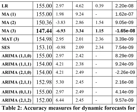
[image:5.612.325.555.91.333.2] [image:5.612.44.281.98.292.2]ARIMA (2,1,2) 152.00 6.44 2.45 - 9.57e-09 0.71 0.02 1.00 1.00 2.11e-06 Table 2: Accuracy measures for dynamic forecasts for
LME copper rate Table 2: Accuracy measures for dynamic forecasts for LME copper rate
AR (0) 148.12 -4.21 3.08 1.65 1.05e-08 0.72 0.02 0.96 0.98 2.32e-06
AR (1) 149.20 -0.80 2.49 1.95 6.03e-09 0.70 0.02 0.97 0.98 1.36e-06
Key:
LR=Linear regression, MA=Moving average,
SES= Single exponential smoothing, MAT=Moving average with trend,
ARIMA=Autoregressive integrated moving average, Std. RSS = Standardized residual sum of squares,
MAE = Mean absolute error,
MAPE = Mean absolute percentage error MSE = Mean square error,