Proceedings of the 2019 Conference on Empirical Methods in Natural Language Processing and the 9th International Joint Conference on Natural Language Processing, pages 55–65,
55
How Contextual are Contextualized Word Representations?
Comparing the Geometry of BERT, ELMo, and GPT-2 Embeddings
Kawin Ethayarajh∗
Stanford University [email protected]
Abstract
Replacing static word embeddings with con-textualized word representations has yielded significant improvements on many NLP tasks. However, just how contextual are the contex-tualized representations produced by models such as ELMo and BERT? Are there infinitely many context-specific representations for each word, or are words essentially assigned one of a finite number of word-sense representations? For one, we find that the contextualized rep-resentations of all words are not isotropic in any layer of the contextualizing model. While representations of the same word in differ-ent contexts still have a greater cosine simi-larity than those of two different words, this self-similarity is much lower in upper layers. This suggests that upper layers of contextu-alizing models produce more context-specific representations, much like how upper layers of LSTMs produce more task-specific repre-sentations. In all layers of ELMo, BERT, and GPT-2, on average, less than 5% of the vari-ance in a word’s contextualized representa-tions can be explained by a static embedding for that word, providing some justification for the success of contextualized representations.
1 Introduction
The application of deep learning methods to NLP is made possible by representing words as vec-tors in a low-dimensional continuous space. Tradi-tionally, these word embeddings werestatic: each word had a single vector, regardless of context (Mikolov et al., 2013a;Pennington et al., 2014). This posed several problems, most notably that all senses of a polysemous word had to share the same representation. More recent work, namely deep neural language models such as ELMo ( Pe-ters et al., 2018) and BERT (Devlin et al.,2018),
∗
Work partly done at the University of Toronto.
have successfully createdcontextualized word rep-resentations, word vectors that are sensitive to the context in which they appear. Replacing static embeddings with contextualized representa-tions has yielded significant improvements on a di-verse array of NLP tasks, ranging from question-answering to coreference resolution.
The success of contextualized word represen-tations suggests that despite being trained with only a language modelling task, they learn highly transferable and task-agnostic properties of lan-guage. In fact, linear probing models trained on frozen contextualized representations can predict linguistic properties of words (e.g., part-of-speech tags) almost as well as state-of-the-art models (Liu et al., 2019a;Hewitt and Manning, 2019). Still, these representations remain poorly understood. For one, just how contextual are these contextu-alized word representations? Are there infinitely many context-specific representations that BERT and ELMo can assign to each word, or are words essentially assigned one of a finite number of word-sense representations?
We answer this question by studying the geom-etry of the representation space for each layer of ELMo, BERT, and GPT-2. Our analysis yields some surprising findings:
represen-tations is surprising.
2. Occurrences of the same word in different contexts have non-identical vector represen-tations. Where vector similarity is defined as cosine similarity, these representations are more dissimilar to each other in upper lay-ers. This suggests that, much like how upper layers of LSTMs produce more task-specific representations (Liu et al.,2019a), upper lay-ers of contextualizing models produce more context-specific representations.
3. Context-specificity manifests very differently in ELMo, BERT, and GPT-2. In ELMo, representations of words in the same sen-tence grow more similar to each other as context-specificity increases in upper layers; in BERT, they become more dissimilar to each other in upper layers but are still more similar than randomly sampled words are on average; in GPT-2, however, words in the same sentence are no more similar to each other than two randomly chosen words.
4. After adjusting for the effect of anisotropy, on average, less than 5% of the variance in a word’s contextualized representations can be explained by their first principal component. This holds across all layers of all models. This suggests that contextualized representa-tions do not correspond to a finite number of word-sense representations, and even in the best possible scenario, static embeddings would be a poor replacement for contextual-ized ones. Still, static embeddings created by taking the first principal component of a word’s contextualized representations out-perform GloVe and FastText embeddings on many word vector benchmarks.
These insights help justify why the use of contex-tualized representations has led to such significant improvements on many NLP tasks.
2 Related Work
Static Word Embeddings Skip-gram with neg-ative sampling (SGNS) (Mikolov et al., 2013a) and GloVe (Pennington et al., 2014) are among the best known models for generating static word embeddings. Though they learn embeddings itera-tively in practice, it has been proven that in theory,
they both implicitly factorize a word-context ma-trix containing a co-occurrence statistic (Levy and Goldberg,2014a,b). Because they create a single representation for each word, a notable problem with static word embeddings is that all senses of a polysemous word must share a single vector.
Contextualized Word Representations Given the limitations of static word embeddings, recent work has tried to create context-sensitive word representations. ELMo (Peters et al.,2018), BERT (Devlin et al.,2018), and GPT-2 (Radford et al.,
2019) are deep neural language models that are fine-tuned to create models for a wide range of downstream NLP tasks. Their internal representa-tions of words are calledcontextualized word rep-resentationsbecause they are a function of the en-tire input sentence. The success of this approach suggests that these representations capture highly transferable and task-agnostic properties of lan-guage (Liu et al.,2019a).
ELMo creates contextualized representations of each token by concatenating the internal states of a 2-layer biLSTM trained on a bidirectional lan-guage modelling task (Peters et al., 2018). In contrast, BERT and GPT-2 are bi-directional and uni-directional transformer-based language mod-els respectively. Each transformer layer of 12-layer BERT (base, cased) and 12-12-layer GPT-2 cre-ates a contextualized representation of each token by attending to different parts of the input sentence (Devlin et al.,2018;Radford et al.,2019). BERT – and subsequent iterations on BERT (Liu et al.,
2019b;Yang et al.,2019) – have achieved state-of-the-art performance on various downstream NLP tasks, ranging from question-answering to senti-ment analysis.
Probing Tasks Prior analysis of contextualized word representations has largely been restricted to probing tasks (Tenney et al.,2019;Hewitt and Manning, 2019). This involves training linear models to predict syntactic (e.g., part-of-speech tag) and semantic (e.g., word relation) proper-ties of words. Probing models are based on the premise that if a simple linear model can be trained to accurately predict a linguistic property, then the representations implicitly encode this information to begin with. While these analyses have found that contextualized representations encode seman-tic and syntacseman-tic information, they cannot answer
what extent they can be replaced with static word embeddings, if at all. Our work in this paper is thus markedly different from most dissections of contextualized representations. It is more similar to Mimno and Thompson (2017), which studied the geometry of static word embedding spaces.
3 Approach
3.1 Contextualizing Models
The contextualizing models we study in this pa-per are ELMo, BERT, and GPT-21. We choose the base cased version of BERT because it is most comparable to GPT-2 with respect to number of layers and dimensionality. The models we work with are all pre-trained on their respective lan-guage modelling tasks. Although ELMo, BERT, and GPT-2 have 2, 12, and 12 hidden layers re-spectively, we also include the input layer of each contextualizing model as its 0th layer. This is be-cause the 0th layer is not contextualized, making
it a useful baseline against which to compare the contextualization done by subsequent layers.
3.2 Data
To analyze contextualized word representations, we need input sentences to feed into our pre-trained models. Our input data come from the SemEval Semantic Textual Similarity tasks from years 2012 - 2016 (Agirre et al.,2012,2013,2014,
2015). We use these datasets because they contain sentences in which the same words appear in dif-ferent contexts. For example, the word ‘dog’ ap-pears in “A panda dog is running on the road.”
and “A dog is trying to get bacon off his back.”
If a model generated the same representation for ‘dog’ in both these sentences, we could infer that there was no contextualization; conversely, if the two representations were different, we could infer that they were contextualized to some extent. Us-ing these datasets, we map words to the list of sen-tences they appear in and their index within these sentences. We do not consider words that appear in less than 5 unique contexts in our analysis.
3.3 Measures of Contextuality
We measure how contextual a word representation is using three different metrics: self-similarity,
intra-sentence similarity, and maximum explain-able variance.
1We use the pretrained models provided in an earlier
ver-sion of thePyTorch-Transformers library.
Definition 1 Let w be a word that appears in sentences{s1, ...,sn} at indices{i1, ...,in}
respec-tively, such thatw=s1[i1] =...=sn[in]. Let f`(s,i)
be a function that mapss[i]to its representation in layer`of model f. Theself similarityofwin layer
`is
SelfSim`(w) = 1 n2−n
∑
j k
∑
6=jcos(f`(sj,ij),f`(sk,ik))
(1) where cos denotes the cosine similarity. In other words, theself-similarityof a wordwin layer`is the average cosine similarity between its contextu-alized representations across itsnunique contexts. If layer ` does not contextualize the representa-tions at all, thenSelfSim`(w) =1 (i.e., the repre-sentations are identical across all contexts). The more contextualized the representations are forw, the lower we would expect its self-similarity to be.
Definition 2 Let s be a sentence that is a se-quence hw1, ...,wni ofn words. Let f`(s,i) be a
function that mapss[i]to its representation in layer
`of model f. Theintra-sentence similarityofsin layer`is
IntraSim`(s) =1
n
∑
i cos(~s`,f`(s,i))where~s`=1
n
∑
i f`(s,i)(2)
Put more simply, theintra-sentence similarityof a sentence is the average cosine similarity between its word representations and the sentence vector, which is just the mean of those word vectors. This measure captures how context-specificity mani-fests in the vector space. For example, if both
IntraSim`(s)andSelfSim`(w)are low∀w∈s, then the model contextualizes words in that layer by giving each one a context-specific representation that is still distinct from all other word represen-tations in the sentence. IfIntraSim`(s)is high but
SelfSim`(w) is low, this suggests a less nuanced contextualization, where words in a sentence are contextualized simply by making their representa-tions converge in vector space.
Definition 3 Let w be a word that appears in sentences{s1, ...,sn} at indices{i1, ...,in}
respec-tively, such thatw=s1[i1] =...=sn[in]. Let f`(s,i)
be a function that mapss[i]to its representation in layer `of model f. Where [f`(s1,i1)...f`(sn,in)]
firstmsingular values of this matrix, themaximum explainable varianceis
MEV`(w) =
σ12
∑iσi2
(3)
MEV`(w)is the proportion of variance inw’s con-textualized representations for a given layer that can be explained by their first principal compo-nent. It gives us an upper bound on how well a static embedding could replace a word’s contex-tualized representations. The closer MEV`(w) is to 0, the poorer a replacement a static embedding would be; ifMEV`(w) =1, then a static
embed-ding would be a perfect replacement for the con-textualized representations.
3.4 Adjusting for Anisotropy
It is important to consider isotropy (or the lack thereof) when discussing contextuality. For ex-ample, if word vectors were perfectly isotropic (i.e., directionally uniform), then SelfSim`(w) =
0.95 would suggest thatw’s representations were poorly contextualized. However, consider the sce-nario where word vectors are so anisotropic that any two words have on average a cosine similar-ity of 0.99. ThenSelfSim`(w) =0.95 would actu-ally suggest the opposite – thatw’s representations were well contextualized. This is because repre-sentations ofwin different contexts would on av-erage be more dissimilar to each other than two randomly chosen words.
To adjust for the effect of anisotropy, we use three anisotropic baselines, one for each of our contextuality measures. For self-similarity and intra-sentence similarity, the baseline is the aver-age cosine similarity between the representations of uniformly randomly sampled words from dif-ferent contexts. The more anisotropic the word representations are in a given layer, the closer this baseline is to 1. For maximum explainable ance (MEV), the baseline is the proportion of vari-ance in uniformly randomly sampled word repre-sentations that is explained by their first principal component. The more anisotropic the representa-tions in a given layer, the closer this baseline is to 1: even for a random assortment of words, the principal component would be able to explain a large proportion of the variance.
Since contextuality measures are calculated for each layer of a contextualizing model, we cal-culate separate baselines for each layer as well.
We then subtract from each measure its respective baseline to get theanisotropy-adjusted contexual-ity measure. For example, the anisotropy-adjusted self-similarity is
Baseline(f`) =Ex,y∼U(O)[cos(f`(x),f`(y))]
SelfSim∗`(w) =SelfSim`(w)−Baseline(f`) (4)
where O is the set of all word occurrences and
f`(·)maps a word occurrence to its representation in layer`of model f. Unless otherwise stated, ref-erences to contextuality measures in the rest of the paper refer to the anisotropy-adjusted measures, where both the raw measure and baseline are esti-mated with 1K uniformly randomly sampled word representations.
4 Findings
4.1 (An)Isotropy
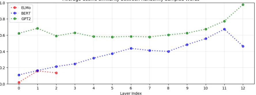
Contextualized representations are anisotropic in all non-input layers. If word representations from a particular layer were isotropic (i.e., direc-tionally uniform), then the average cosine similar-ity between uniformly randomly sampled words would be 0 (Arora et al., 2017). The closer this average is to 1, the more anisotropic the represen-tations. The geometric interpretation of anisotropy is that the word representations all occupy a nar-row cone in the vector space rather than being uni-form in all directions; the greater the anisotropy, the narrower this cone (Mimno and Thompson,
2017). As seen in Figure 1, this implies that in almost all layers of BERT, ELMo and GPT-2, the representations of all words occupy a narrow cone in the vector space. The only exception is ELMo’s input layer, which produces static character-level embeddings without using contextual or even po-sitional information (Peters et al.,2018). It should be noted that not all static embeddings are neces-sarily isotropic, however; Mimno and Thompson
(2017) found that skipgram embeddings, which are also static, are not isotropic.
Figure 1: In almost all layers of BERT, ELMo, and GPT-2, the word representations are anisotropic (i.e., not directionally uniform): the average cosine similarity between uniformly randomly sampled words is non-zero. The one exception is ELMo’s input layer; this is not surprising given that it generates character-level embeddings without using context. Representations in higher layers are generally more anisotropic than those in lower ones.
ELMo as well, though there are exceptions: for ex-ample, the anisotropy in BERT’s penultimate layer is much higher than in its final layer.
Isotropy has both theoretical and empirical ben-efits for static word embeddings. In theory, it allows for stronger “self-normalization” during training (Arora et al.,2017), and in practice, sub-tracting the mean vector from static embeddings leads to improvements on several downstream NLP tasks (Mu et al., 2018). Thus the extreme degree of anisotropy seen in contextualized word representations – particularly in higher layers – is surprising. As seen in Figure 1, for all three models, the contextualized hidden layer represen-tations are almost all more anisotropic than the in-put layer representations, which do not incorpo-rate context. This suggests that high anisotropy is inherent to, or least a by-product of, the process of contextualization.
4.2 Context-Specificity
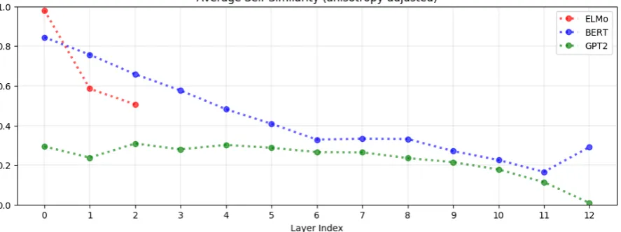
Contextualized word representations are more context-specific in higher layers. Recall from Definition 1 that the self-similarity of a word, in a given layer of a given model, is the average co-sine similarity between its representations in dif-ferent contexts, adjusted for anisotropy. If the self-similarity is 1, then the representations are not context-specific at all; if the self-similarity is 0, that the representations are maximally context-specific. In Figure 2, we plot the average self-similarity of uniformly randomly sampled words
in each layer of BERT, ELMo, and GPT-2. For example, the self-similarity is 1.0 in ELMo’s in-put layer because representations in that layer are static character-level embeddings.
In all three models, the higher the layer, the lower the self-similarity is on average. In other words, the higher the layer, the more context-specific the contextualized representations. This finding makes intuitive sense. In image classifica-tion models, lower layers recognize more generic features such as edges while upper layers recog-nize more class-specific features (Yosinski et al.,
2014). Similarly, upper layers of LSTMs trained on NLP tasks learn more task-specific represen-tations (Liu et al., 2019a). Therefore, it fol-lows that upper layers of neural language mod-els learn more context-specific representations, so as to predict the next word for a given context more accurately. Of all three models, representa-tions in GPT-2 are the most context-specific, with those in GPT-2’s last layer being almost maxi-mally context-specific.
Figure 2: The average cosine similarity between representations of the same word in different contexts is called the word’sself-similarity(see Definition 1). Above, we plot the average self-similarity of uniformly randomly sampled words after adjusting for anisotropy (see section3.4). In all three models, the higher the layer, the lower the self-similarity, suggesting that contextualized word representations are more context-specific in higher layers.
of contexts a word appears in, rather than its inher-ent polysemy, is what drives variation in its con-textualized representations. This answers one of the questions we posed in the introduction: ELMo, BERT, and GPT-2 are not simply assigning one of a finite number of word-sense representations to each word; otherwise, there would not be so much variation in the representations of words with so few word senses.
Context-specificity manifests very differently in ELMo, BERT, and GPT-2. As noted earlier, contextualized representations are more context-specific in upper layers of ELMo, BERT, and GPT-2. However, how does this increased context-specificity manifest in the vector space? Do word representations in the same sentence converge to a single point, or do they remain distinct from one another while still being distinct from their repre-sentations in other contexts? To answer this ques-tion, we can measure a sentence’s intra-sentence similarity. Recall from Definition 2 that the intra-sentence similarity of a intra-sentence, in a given layer of a given model, is the average cosine similarity between each of its word representations and their mean, adjusted for anisotropy. In Figure3, we plot the average intra-sentence similarity of 500 uni-formly randomly sampled sentences.
In ELMo, words in the same sentence are more similar to one another in upper layers. As word representations in a sentence become more context-specific in upper layers, the intra-sentence
similarity also rises. This suggests that, in prac-tice, ELMo ends up extending the intuition behind Firth’s (1957) distributional hypothesis to the tence level: that because words in the same sen-tence share the same context, their contextualized representations should also be similar.
In BERT, words in the same sentence are more dissimilar to one another in upper layers. As word representations in a sentence become more context-specific in upper layers, they drift away from one another, although there are exceptions (see layer 12 in Figure 3). However, in all lay-ers, the average similarity between words in the same sentence is still greater than the average sim-ilarity between randomly chosen words (i.e., the anisotropy baseline). This suggests a more nu-anced contextualization than in ELMo, with BERT recognizing that although the surrounding sen-tence informs a word’s meaning, two words in the same sentence do not necessarily have a similar meaning because they share the same context.
Figure 3: The intra-sentence similarityis the average cosine similarity between each word representation in a sentence and their mean (see Definition 2). Above, we plot the average intra-sentence similarity of uniformly randomly sampled sentences, adjusted for anisotropy. This statistic reflects how context-specificity manifests in the representation space, and as seen above, it manifests very differently for ELMo, BERT, and GPT-2.
average intra-sentence similarity is above 0.20 for all but one layer.
As noted earlier when discussing BERT, this be-havior still makes intuitive sense: two words in the same sentence do not necessarily have a similar meaning simply because they share the same con-text. The success of GPT-2 suggests that unlike anisotropy, which accompanies context-specificity in all three models, a high intra-sentence similar-ity is not inherent to contextualization. Words in the same sentence can have highly contextualized representations without those representations be-ing any more similar to each other than two ran-dom word representations. It is unclear, however, whether these differences in intra-sentence simi-larity can be traced back to differences in model architecture; we leave this question as future work.
4.3 Static vs. Contextualized
On average, less than 5% of the variance in a word’s contextualized representations can be explained by a static embedding. Recall from Definition 3 that the maximum explainable vari-ance(MEV) of a word, for a given layer of a given model, is the proportion of variance in its con-textualized representations that can be explained by their first principal component. This gives us an upper bound on how well a static embedding could replace a word’s contextualized representa-tions. Because contextualized representations are anisotropic (see section 4.1), much of the varia-tion across all words can be explained by a
sin-gle vector. We adjust for anisotropy by calculating the proportion of variance explained by the first principal component of uniformly randomly sam-pled word representations and subtracting this pro-portion from the raw MEV. In Figure4, we plot the average anisotropy-adjusted MEV across uni-formly randomly sampled words.
In no layer of ELMo, BERT, or GPT-2 can more than 5% of the variance in a word’s contextual-ized representations be explained by a static em-bedding, on average. Though not visible in Figure
4, the raw MEV of many words is actually below the anisotropy baseline: i.e., a greater proportion of the variance across all words can be explained by a single vector than can the variance across all representations of a single word. Note that the 5% threshold represents the best-case scenario, and there is no theoretical guarantee that a word vector obtained using GloVe, for example, would be similar to the static embedding that maximizes MEV. This suggests that contextualizing models are not simply assigning one of a finite number of word-sense representations to each word – other-wise, the proportion of variance explained would be much higher. Even the average raw MEV is be-low 5% for all layers of ELMo and BERT; only for GPT-2 is the raw MEV non-negligible, being around 30% on average for layers 2 to 11 due to extremely high anisotropy.
Figure 4: Themaximum explainable variance(MEV) of a word is the proportion of variance in its contextualized representations that can be explained by their first principal component (see Definition 3). Above, we plot the average MEV of uniformly randomly sampled words after adjusting for anisotropy. In no layer of any model can more than 5% of the variance in a word’s contextualized representations be explained by a static embedding.
Static Embedding SimLex999 MEN WS353 RW Google MSR SemEval2012(2) BLESS AP
GloVe 0.194 0.216 0.339 0.127 0.189 0.312 0.097 0.390 0.308
FastText 0.239 0.239 0.432 0.176 0.203 0.289 0.104 0.375 0.291
ELMo, Layer 1 0.276 0.167 0.317 0.148 0.170 0.326 0.114 0.410 0.308
ELMo, Layer 2 0.215 0.151 0.272 0.133 0.130 0.268 0.132 0.395 0.318
BERT, Layer 1 0.315 0.200 0.394 0.208 0.236 0.389 0.166 0.365 0.321
BERT, Layer 2 0.320 0.166 0.383 0.188 0.230 0.385 0.149 0.365 0.321
BERT, Layer 11 0.221 0.076 0.319 0.135 0.175 0.290 0.149 0.370 0.289
BERT, Layer 12 0.233 0.082 0.325 0.144 0.184 0.307 0.144 0.360 0.294
GPT-2, Layer 1 0.174 0.012 0.176 0.183 0.052 0.081 0.033 0.220 0.184
GPT-2, Layer 2 0.135 0.036 0.171 0.180 0.045 0.062 0.021 0.245 0.184
GPT-2, Layer 11 0.126 0.034 0.165 0.182 0.031 0.038 0.045 0.270 0.189 GPT-2, Layer 12 0.140 -0.009 0.113 0.163 0.020 0.021 0.014 0.225 0.172
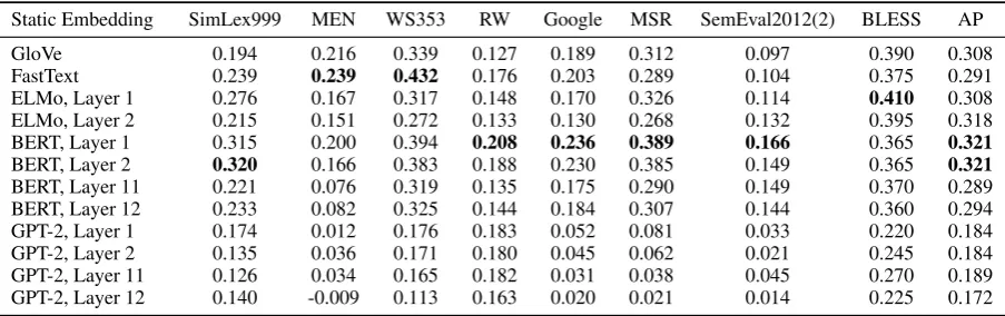
Table 1: The performance of various static embeddings on word embedding benchmark tasks. The best result for each task is in bold. For the contextualizing models (ELMo, BERT, GPT-2), we use the first principal component of a word’s contextualized representations in a given layer as its static embedding. The static embeddings created using ELMo and BERT’s contextualized representations often outperform GloVe and FastText vectors.
earlier, we can create static embeddings for each word by taking the first principal component (PC) of its contextualized representations in a given layer. In Table 1, we plot the performance of thesePC static embeddingson several benchmark tasks2. These tasks cover semantic similarity,
analogy solving, and concept categorization: Sim-Lex999 (Hill et al., 2015), MEN (Bruni et al.,
2014), WS353 (Finkelstein et al.,2002), RW ( Lu-ong et al., 2013), SemEval-2012 (Jurgens et al.,
2012), Google analogy solving (Mikolov et al.,
2013a) MSR analogy solving (Mikolov et al.,
2013b), BLESS (Baroni and Lenci,2011) and AP (Almuhareb and Poesio,2004). We leave out lay-ers 3 - 10 in Table1because their performance is
2TheWord Embeddings Benchmarkspackage was used
for evaluation.
between those of Layers 2 and 11.
[image:8.595.73.525.313.455.2]represen-tations, such as those from Layer 1 of BERT, are much more effective.
5 Future Work
Our findings offer some new directions for future work. For one, as noted earlier in the paper, Mu et al.(2018) found that making static embeddings more isotropic – by subtracting their mean from each embedding – leads to surprisingly large im-provements in performance on downstream tasks. Given that isotropy has benefits for static embed-dings, it may also have benefits for contextual-ized word representations, although the latter have already yielded significant improvements despite being highly anisotropic. Therefore, adding an anisotropy penalty to the language modelling ob-jective – to encourage the contextualized represen-tations to be more isotropic – may yield even better results.
Another direction for future work is generat-ing static word representations from contextual-ized ones. While the latter offer superior per-formance, there are often challenges to deploying large models such as BERT in production, both with respect to memory and run-time. In contrast, static representations are much easier to deploy. Our work in section 4.3 suggests that not only it is possible to extract static representations from con-textualizing models, but that these extracted vec-tors often perform much better on a diverse array of tasks compared to traditional static embeddings such as GloVe and FastText. This may be a means of extracting some use from contextualizing mod-els without incurring the full cost of using them in production.
6 Conclusion
In this paper, we investigated how contextual con-textualized word representations truly are. For one, we found that upper layers of ELMo, BERT, and GPT-2 produce more context-specific rep-resentations than lower layers. This increased context-specificity is always accompanied by in-creased anisotropy. However, context-specificity also manifests differently across the three models; the anisotropy-adjusted similarity between words in the same sentence is highest in ELMo but al-most non-existent in GPT-2. We ultimately found that after adjusting for anisotropy, on average, less than 5% of the variance in a word’s contextual-ized representations could be explained by a static
embedding. This means that even in the best-case scenario, in all layers of all models, static word embeddings would be a poor replacement for con-textualized ones. These insights help explain some of the remarkable success that contextualized rep-resentations have had on a diverse array of NLP tasks.
Acknowledgments
We thank the anonymous reviewers for their in-sightful comments. We thank the Natural Sciences and Engineering Research Council of Canada (NSERC) for their financial support.
References
Eneko Agirre, Carmen Banea, Claire Cardie, Daniel M Cer, Mona T Diab, Aitor Gonzalez-Agirre, Weiwei Guo, Inigo Lopez-Gazpio, Montse Maritxalar, Rada Mihalcea, et al. 2015. Semeval-2015 task 2: Seman-tic textual similarity, English, Spanish and pilot on interpretability. InProceedings SemEval@ NAACL-HLT. pages 252–263.
Eneko Agirre, Carmen Banea, Claire Cardie, Daniel M Cer, Mona T Diab, Aitor Gonzalez-Agirre, Weiwei Guo, Rada Mihalcea, German Rigau, and Janyce Wiebe. 2014. Semeval-2014 task 10: Multilin-gual semantic textual similarity. InProceedings Se-mEval@ COLING. pages 81–91.
Eneko Agirre, Daniel Cer, Mona Diab, Aitor Gonzalez-Agirre, and Weiwei Guo. 2013. Sem 2013 shared task: Semantic textual similarity, including a pilot on typed-similarity. InSEM 2013: The Second Joint Conference on Lexical and Computational Seman-tics. Association for Computational Linguistics.
Eneko Agirre, Mona Diab, Daniel Cer, and Aitor Gonzalez-Agirre. 2012. Semeval-2012 task 6: A pi-lot on semantic textual similarity. In Proceedings of the First Joint Conference on Lexical and Com-putational Semantics-Volume 1: Proceedings of the main conference and the shared task, and Volume 2: Proceedings of the Sixth International Workshop on Semantic Evaluation. Association for Computa-tional Linguistics, pages 385–393.
Abdulrahman Almuhareb and Massimo Poesio. 2004. Attribute-based and value-based clustering: An evaluation. InProceedings of the 2004 conference on empirical methods in natural language process-ing.
Marco Baroni and Alessandro Lenci. 2011. How we blessed distributional semantic evaluation. In Pro-ceedings of the GEMS 2011 Workshop on GEomet-rical Models of Natural Language Semantics. Asso-ciation for Computational Linguistics, pages 1–10.
Elia Bruni, Nam-Khanh Tran, and Marco Baroni. 2014. Multimodal distributional semantics. Journal of Ar-tificial Intelligence Research49:1–47.
Jacob Devlin, Ming-Wei Chang, Kenton Lee, and Kristina Toutanova. 2018. Bert: Pre-training of deep bidirectional transformers for language understand-ing. arXiv preprint arXiv:1810.04805.
Lev Finkelstein, Evgeniy Gabrilovich, Yossi Matias, Ehud Rivlin, Zach Solan, Gadi Wolfman, and Ey-tan Ruppin. 2002. Placing search in context: The concept revisited. ACM Transactions on informa-tion systems20(1):116–131.
John R Firth. 1957. A synopsis of linguistic theory, 1930-1955. Studies in linguistic analysis.
John Hewitt and Christopher D. Manning. 2019. A structural probe for finding syntax in word represen-tations. In North American Chapter of the Associ-ation for ComputAssoci-ational Linguistics: Human Lan-guage Technologies. Association for Computational Linguistics.
Felix Hill, Roi Reichart, and Anna Korhonen. 2015. Simlex-999: Evaluating semantic models with (gen-uine) similarity estimation. Computational Linguis-tics41(4):665–695.
David A Jurgens, Peter D Turney, Saif M Mohammad, and Keith J Holyoak. 2012. Semeval-2012 task 2: Measuring degrees of relational similarity. In Pro-ceedings of the First Joint Conference on Lexical and Computational Semantics-Volume 1: Proceed-ings of the main conference and the shared task, and Volume 2: Proceedings of the Sixth International Workshop on Semantic Evaluation. Association for Computational Linguistics, pages 356–364.
Omer Levy and Yoav Goldberg. 2014a. Linguistic reg-ularities in sparse and explicit word representations. InProceedings of the eighteenth conference on com-putational natural language learning. pages 171– 180.
Omer Levy and Yoav Goldberg. 2014b. Neural word embedding as implicit matrix factorization. In Ad-vances in Neural Information Processing Systems. pages 2177–2185.
Nelson F. Liu, Matt Gardner, Yonatan Belinkov, Matthew E. Peters, and Noah A. Smith. 2019a. Lin-guistic knowledge and transferability of contextual representations. InProceedings of the Conference of the North American Chapter of the Association for Computational Linguistics: Human Language Tech-nologies.
Yinhan Liu, Myle Ott, Naman Goyal, Jingfei Du, Man-dar Joshi, Danqi Chen, Omer Levy, Mike Lewis, Luke Zettlemoyer, and Veselin Stoyanov. 2019b. Roberta: A robustly optimized bert pretraining ap-proach. arXiv preprint arXiv:1907.11692.
Thang Luong, Richard Socher, and Christopher D Manning. 2013. Better word representations with recursive neural networks for morphology. In
SIGNLL Conference on Computational Natural Language Learning (CoNLL). pages 104–113.
Tomas Mikolov, Ilya Sutskever, Kai Chen, Greg S Cor-rado, and Jeff Dean. 2013a. Distributed representa-tions of words and phrases and their compositional-ity. InAdvances in Neural Information Processing Systems. pages 3111–3119.
Tomas Mikolov, Wen-tau Yih, and Geoffrey Zweig. 2013b. Linguistic regularities in continuous space word representations. InProceedings of the 2013 Conference of the North American Chapter of the Association for Computational Linguistics: Human Language Technologies. pages 746–751.
David Mimno and Laure Thompson. 2017. The strange geometry of skip-gram with negative sampling. In
Proceedings of the 2017 Conference on Empirical Methods in Natural Language Processing. pages 2873–2878.
Jiaqi Mu, Suma Bhat, and Pramod Viswanath. 2018. All-but-the-top: Simple and effective postprocess-ing for word representations. InProceedings of the 7th International Conference on Learning Represen-tations (ICLR).
Jeffrey Pennington, Richard Socher, and Christopher Manning. 2014. GloVe: Global vectors for word representation. In Proceedings of the 2014 Con-ference on Empirical Methods in Natural Language Processing (EMNLP). pages 1532–1543.
Matthew Peters, Mark Neumann, Mohit Iyyer, Matt Gardner, Christopher Clark, Kenton Lee, and Luke Zettlemoyer. 2018. Deep contextualized word rep-resentations. In Proceedings of the 2018 Confer-ence of the North American Chapter of the Associ-ation for ComputAssoci-ational Linguistics: Human Lan-guage Technologies, Volume 1 (Long Papers). pages 2227–2237.
Alec Radford, Jeff Wu, Rewon Child, David Luan, Dario Amodei, and Ilya Sutskever. 2019. Language models are unsupervised multitask learners .
Ian Tenney, Patrick Xia, Berlin Chen, Alex Wang, Adam Poliak, R. Thomas McCoy, Najoung Kim, Benjamin Van Durme, Samuel R. Bowman, Dipan-jan Das, and Ellie Pavlick. 2019. What do you learn from context? probing for sentence structure in contextualized word representations. In Inter-national Conference on Learning Representations.
Zhilin Yang, Zihang Dai, Yiming Yang, Jaime Car-bonell, Ruslan Salakhutdinov, and Quoc V Le. 2019. Xlnet: Generalized autoregressive pretrain-ing for language understandpretrain-ing. arXiv preprint arXiv:1906.08237.