Avant-Garde Matrix Splitting for the Solution of Sparse Non-symmetric Linear Systems

(1)

Avant-Garde Matrix Splitting for the Solution of

Sparse Non-symmetric Linear Systems

A. A. Shah

Institute of Business Administration, City Campus, Garden/Kiyani Shaheed Road, Karachi. [email protected]

Abstract--A non-symmetric matrix splitting is presented for the solution of certain sparse linear systems. The author reports the comparison and the convergence performance of the previous and the contemporary methods and includes explicit comments. It is studied that some recent methods may work efficiently with a symmetric matrix but show insufficiencies like numerical instability and non-scaling invariant with non-symmetric matrix. The proposed matrix splitting can overcome these deficiencies.

Keywords: Sparse matrix, M-matrices,

orthogonalization, Krylov Space, Iterative Methods

1-Introduction.

Recently some orthogonalization iterative methods e.g. GMRES methods or generalized minimal residual methods have been used for the solution of sparse symmetric linear systems,

Ax = b ……….(1.1)

Where A is a sparse matrix. In most of the studies these methods are matched up to and compared in many studies (see, for example [2],

[3], [15], [16], [17] and [19]). These methods in

fact minimize rn = b – Axn = nth residual in a

Krylov Space Kn(A;r0). With an initial

presumption x0 an inimitable sequence {xn} is

created with:

xn x0 + < Ar0, A2r0, A3r0, A4r0 ……. ,

An-1_r

0 > …………..(1.2)

satisfying:

rn = minimum, ………(1.3)

which is equivalent to the orthogonality condition:

rn ⊥ < Ar0, A2r0, A3r0, A4r0 ……. , An-1r0 >

………..(1.4)

The vigorous execution of (1.2) – (1.4) is

GMRES iteration method. The execution uses

Arnoldi Method (see [1]) to create an orthogonal basis for the Krylov Space Kn(A;r0) which leads

to an (n + 1) x n Hessenberg Least-Square problem ( see [16]). At each step we have: en =

pn(A)e0 , rn = pn(A)r0 where pn(Z) is a

polynomial of degree n with and pn(0) = 1.

Convergence will take place if and only if pn

exists for which ║pn(A)r0║decreases rapidly,

and a sufficient condition for this is that

║pn(A)║should decrease rapidly. GMRES is in

fact well suited to normal matrices unfortunately nonsymmetric matrices are rarely normal. There is always storage requirement problem and to keep storage requirement under control,

GMRES is often restarted after each k- steps

(see [15]). It is also reported that GMRES algorithm is unreliable as there are instances where the residual norms produced by the algorithm, although non-increasing, do not converge to zero (see [16]). As far as the

GMRES-Like methods, for example BCG

method and a sufficient condition for this is that

║pn(A)║should decrease rapidly. GMRES is in

fact well suited to normal matrices and unfortunately nonsymmetric matrices are rarely normal. There is always storage requirement problem and to keep storage requirement under control, GMRES is often restarted after each

k-steps (see [15]). It is also reported that GMRES

algorithm is unreliable as there are instances where the residual norms produced by the algorithm, although non-increasing, do not converge to zero (see [16]). As far as the

GMRES-Like methods, for example BCG

method and CGS methods, are concerned it is reported that they are susceptible to the possibility of breakdown-division by zero (see

[15]). Gutknecht ([9]) has presented a

BICGStab method for matrices with complex

spectrum.

(2)

)

y

-

(0)

x

(A

T

A

i - 1

A)

T

(A

k

i

1 i

i

α

(0)

x

(k)

x

∑

=

+

=

where α is chosen to minimize

x

(k)

-

x

. The main problem with this approach is that the amount of work per iteration is almost doubled because it is necessary to multiply by AT and A at each iteration in order to avoid the actual production of ATA in the sparse case. It can be noted that when A is not symmetric

( )

2

1 T

_A

A

may be a poor approximation to AT or A and, therefore,

( )

2

1 T

_A

A

cannot be used in place of A. In other studies more importance is given to the splitting of the coefficient matrix, which draws to a close to the storage problem and provides reliable methods for the solution of non-symmetric systems (see [17] and [13]). We present the results and findings of one of these studies for a general reader. The computer codes of the method are published. We also present some new theorems which are proved recently. The method is designed for the solution of non-symmetric systems (1.1) but it is capable of using all the robust techniques, developed for the solution of symmetric linear systems. The method is found to be more suitable for the iterative solution of (1.1), where A is a sparse unsymmetric M-matrix or nearly symmetric structured M-matrix. We propose a particular class of regular splitting and call this class of regular splitting the generalized regular splitting or GRS and the corresponding iterative method, the generalized regular splitting method or GRSI method. A simple technique is designed to produce a symmetric and positive definite matrix or SPD splitting matrix. This allows for the stable efficient incomplete Cholesky factorization of the splitting matrix as the preliminary steps to an iterative solution. Because of the presence of a SPD matrix any other efficient technique developed for symmetric system can be used.

Definition1.1:

Given an M-matrix A, the splitting

A = (S + ∆) - (H + ∆)………...…(1.2)

Is called the generalized regular splitting or GRS if S = [si,j] is a symmetric M-matrix such

that:

The matrix H = [hi,j] is such that

hi,j = si,j - ai,j ≥ 0 for all i,j.

The non-negative diagonal matrix Δ = [δi,j] is

such that:

2- Choice of δ.

If matrix S is not a diagonally dominant matrix, a non-negative diagonal matrix Δ = [δi,j] is added

to make the matrix S a diagonally dominant matrix to avoid the breakdown, where δis small and is chosen so that (S + ∆) is a symmetric and diagonally dominant M-matrix and (H + ∆)≥ 0. A simple choice of δcould be as follows:

i

j

,

10 ii

a

n

1 j

max

-7

n 1,...., i

≠

∀

+

⎟

⎠

⎞

⎜

⎝

⎛ ∑

₌

=

a

ij

δ

Such matrices (S + ∆) can be easily factorized in a stable manner into incomplete Cholesky factors (see, for example, [14]). It is noted that the smaller the ∆ the faster the convergence of the GRSI method.

3- Description of the algorithm.

Let us consider the system Ax = b, where A =

[ai,j] is a sparse nonsymmetric, N x N,

M-matrix . Let

A = (S + ∆) - (H` + ∆)………..(3.1)

be the GRS of A.

As (S + ∆) is a symmetric and diagonally

dominant M-matrix it can be decomposed into triangular factors or incomplete Cholesky factors i.e. (S + ∆) = LDLT – E is a regular splitting (see

[14]), where E is computed explicitly.

It then follows that A = LDLT – (H` + E + ∆) is a regular splitting. Substituting H for H` + E the iterative system can be written:

,

n

k

,

x

)

(H

b

x

( ) ( 1)

>

<

∈

Δ

+

=

k−

k T

LDL

where x(0) is arbitrary. Substituting the values of

x(k-1)

in turn we obtain,

x(k)_{= [ I + {(LDL}T₎-1_{(H +}_∆_{)} + {(LDL}T₎-1_(H

+ ∆)}2_{+ {(LDL}T₎-1_{(H +}_∆_)}3_{+ ………...}₊

{(LDLT₎-1_{(H +}_∆_)}(k-1)_](LDLT₎-1_{b +{(LDL}T₎-1_(H

+ ∆)}k _x(0)_{………..………(3.2)}

j , i

s

=

{

max{ai,j, aj,I)

_if

_i

_≠

_j

ai,j

_if

_{i = j}

j , i

δ

=

{

0

if

i

≠

j

(3)

If G = {(LDLT)-1(H + ∆)} then, x(k) = [ I +

G + G2_{+ G}3_{+ G}4_{…… + G}(k-1)_](LDLT₎-1_b

+ + Gk_x(0)_{…….……….(3.3)}

Moreover x(k) → A-1b,

i.e. the solution of the linear system because the spectral radius ρ(G) is less than one, so that

G(k) _→₀

and as k → ∞,

. 1 -G) (I ] 1 -k

0 p

p G

[ ∑ →

=

A number of authors like [7] and [11] have devised similar splittings for the case when A is a large sparse singular and irreducible M-matrix. They also worked with nearly symmetric matrices, which they define as having a symmetric, zero structure. The splitting matrix is constructed to be symmetric by dropping terms from A and, as a result, the direct part of the direct iterative method can take advantage of (i) symmetric pivoting (ii) a standard symmetric ordering scheme and (iii) a static storage scheme for the factor L. The author reports that the direct-iterative method is faster than straightforward iteration with the Gauss-Seidel method. The splitting we propose has similar advantages but no terms from A are dropped.

4-Convergence

The GRSI method associated with the GRS splitting is given by

b

x

H

x

S

+

Δ

(k)

=

+

Δ

(k−1)

+

)

(

)

(

or

b

S

x

H

S

x

k k

1

) 1 ( 1

) (

)

(

)

(

)

(

−

− −

Δ

+

Δ

+

Δ

+

=

or

x

(k)

=

G

x

(k−1)

+

η

where the iteration matrix is given by

)

(

)

(

₊

_Δ

1

₊

_Δ

=

_S

−

_H

G

and

b

S

₎

1

(

+

Δ

−

=

η

.

Theorem 4-1: ([18], p.89).

If A = P – Q is a regular splitting of matrix A

and A-1

≥

0, then

ρ

(P-1_Q)=

ρ

_(A-1_Q)/(1+

ρ

_(A-1_{Q)<1 (4.1)}

i.e. the matrix P-1Q is convergent, and the

iterative method

b

P

x

Q

P

x

(k) 1 (k 1) 1

)

(

− −

+

−

=

converges for

any initial value

x

(0)

of

x

if (4.1) is satisfied.

Theorem 4-2:

The spectral radius of the iteration matrix of GRSI method is less than 1, and hence the method converges for any initial value

x

of

x

(0) when the coefficient matrix A is an M-matrix.

Proof: Follows directly from theorem 4-1 since GRS is a regular splitting and A-1

≥

0.

Lemma 4-1:

The iteration matrix G of the GRSI method is a non-negative matrix when A is an M-matrix. Proof: A =

(

S

+

Δ

)

−

(

H

+

Δ

)

Now

(

S

+

Δ

)

−1

≥

0

as

)

(

S

+

Δ

is an M-matrix

And

(

H

+

Δ

)

≥

0

therefore,

)

(

)

(

₊

_Δ

1

₊

_Δ

=

_S

−

_H

G

≥

0 .

Theorem 4-3: ([20], p 125)

Let A be a monotone matrix and let A = Q1 – R1

and A = Q2 – R2 be two regular splittings of A.

If R2

≤

R1, then

(

)

(

₁

)

1 1 2

1

2

R

S

Q

R

Q

S

−

≤

− .

Theorem 4-4. The smaller is the

δ

the faster is

the convergence of the GRSI method. Proof: Obvious from theorem 4-3.

Theorem 4-5. Let A = [ai,j] be an N x N

non-symmetric M-matrix and

x

≥

0

be any non-zero

vector such that

⎭

⎬

⎫

⎩

⎨

⎧

=

∑

=

n

j

i j j i

x

a

x

r

1

,

/

min

.

If A =

(

S

+

Δ

)

−

(

H

+

Δ

)

is a GRS of A, then

α

β

≥

, where

β

is any eigenvalue of

)

(

S

+

Δ

and

{ }

r

_x

x

0

0 sup

≠

≥

=

α

.

Proof:

A=

(

S

+

Δ

)

−

(

H

+

Δ

)

⇒

)

(

)

(

)

(

_S

₊

_Δ

−1

_A

₌

_I

₋

_S

₊

_Δ

−1

_H

₊

_Δ

= I – G.

i.e.

G

=

I

−

(

S

+

Δ

)

−1

A

and by Lemma 4-1

G

≥

0

.

i.e.

[

I

−

(

S

+

Δ

)

−1

A

]

A

−1

≥

0 ⇒

A

−1

≥

0 .

i.e.

A

−1

−

(

S

+

Δ

)

−1

≥

0

, by definition 1.1

1

₍

₎

−

_≥

_S

₊

_Δ

A

.

By theorem 4-3,

1

1 β

α

.

β

α

≥

⇒

≥

Theorem 4-6. Let G = [gi,j]

≥

0 be an N x N

(4)

⎥

⎦

⎤

⎢

⎣

⎡

≤

<

⎥

⎦

⎤

⎢

⎣

⎡

≤

∑

= = i n j j j i i n j j j i

x

g

n

i

G

x

g

n

i

1 , max 1 , min

1 )

(

1 ρ

or

)

(

1 ,

G

x

g

i n

j i j j

₌

_ρ

⎥

⎦

⎤

⎢

⎣

⎡

_∑

= . Moreover,

⎪

⎭

⎪

⎬

⎫

⎪

⎩

⎪

⎨

⎧

⎥

⎦

⎤

⎢

⎣

⎡

≤

∈

=

⎪

⎭

⎪

⎬

⎫

⎪

⎩

⎪

⎨

⎧

⎥

⎦

⎤

⎢

⎣

⎡

≤

∈

∑

= = i n j j j i i n

j i j j

x

g

n

i

P

x

G

x

g

n

i

P

x

1 , max inf * 1 , min sup *

1 )

(

1 ρ

Proof: Follows the steps of theorem 2.2 of

(Varga [1962], p.32).

Each upper and lower bound for the spectral radius of the iteration matrix of the GRSI method can thus be obtained by simple arithmetic steps.

5-Comparison with the standard methods.

There are economical and efficient techniques for the solution of linear symmetric systems. Furthermore, the situation regarding the availability of software implementing iterative schemes for symmetric systems is also satisfactory. As mentioned earlier these techniques for the solution of symmetric systems cannot be extended to the case of nonsymmetric linear systems. As far as the availability of the software is concerned apart from the codes of Paige and Saunders most are experimental. The packages like SPARSPAK (see Geogge and Liu, 1980) and the Yale

Sparse Matrix Package (see Duff and Reid,

1983) are numerically sound if the coefficient matrix in a system of linear equations is SPD. If it is not, the packages may still be used but may

be numerically unsound (see [13]). The GRSIM subroutine is designed to use the ease and comfort of all the efficient methods currently solving symmetric systems of linear equations, for the solution of nonsymmetric systems. Any technique, which can solve a symmetric system easily and economically, can be incorporated to

the GRSI method to form a pristine version of

the GRSI method e.g. the GRSI Cholesky

factorization or GRSI-CF version and the GRSI Incomplete Cholesky factorization or GRSI-ICF version. The method uses a regular splitting. Therefore the convergence is guaranteed. For an unsymmetric M-matrix it can be easily proved numerically that the GRSI method converges faster than the Jacobi and Gauss-Seidel methods.

The GRSI method is not compared with the

direct solution method of the unsymmetric system because of the fact that the direct solution method is only about twice as expensive as a Cholesky factorization (see [6]).

6-Numerical Testing.

We illustrate the numerical behaviour of the

GRSI method by the following simple examples.

In most of the experiments we consider the linear elliptic equation:

au×x + cuyy + dux + euy + fu = g(x,y)

………...(6.1)

in the rectangular region R: 0 ≤ x ≤α, 0 ≤ y ≤β, with Dirichlet boundary conditions. We suppose, for definiteness, that a > 0, b > 0 and f ≤ 0 and all are bounded in the region R and on its boundary B. Upon employing second-order central difference procedures, the finite-difference approximation for the above equation becomes: β1Ui+1,j + β2Ui-1,j + β3Ui,j+1 + β4Ui,j-1 - β0Ui,j = h2gi,j

whereβiare functions of xi = ih, yi = jh,

given by β0 = 2(ai,j + ci,j - ½h2fi,j), β1 = ai,j +

½hdi,j, β2 = ai,j - ½hdi,j, β3 = ci,j + ½hei,j, β4

= ci,j - ½hei,j. The notation ai,j refer to a(ih, jh),

evaluated at the point where the computational module is centered. The coefficient matrix A, so obtained is an irreducible M-matrix.

Example-1.

(5)

necessary for the estimation of the iteration-parameter for the SOR method and the work for the decomposition of the GRSI matrix into Incomplete Cholesky factors has been neglected. This work will in general be small compared to the computational work needed to carry out the actual iterations. Accurate determination of the SOR parameter may be difficult in some circumstances.

TABLE -1

Approximate Number of Multiplication Operation needed for

one iteration in the solution of Ax = b (A is an N X N matrix)

Method No. of

Operations

SOR 6N Gauss-Seidel 5N

Jacobi 5N GRSI 7N

A number of nonsymmetric linear systems of equations were obtained by using the natural mesh ordering and discretizing (6.1) with arbitrary values of the coefficients a, c, d, e, f and the mesh size h. A comparison on the basis of asymptotic rate of convergence of the

GRSI-CF, the GRSI-ICF, the Jacobi, the

Gauss-Seidel and the SOR methods was made. We

report a few of these results. The matrix ∆ is considered to be a zero matrix and the optimum parameter for SOR is used through out.

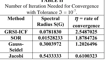
Example-2. We considered a BST matrix with

[image:5.612.91.295.484.610.2]

known sparsity and eigenvalues. The result is given in the following table.

TABLE II

Number of Iteration Needed for Convergence with Tolerance ℑ = 10-7.

Method Spectral

Radius S(G) _convergence

η

= rate of GRSI-ICF 0.0781830 2.5487025

SOR 0.01528233 1.8784726

Gauss-Seidel

0.3003972 1.2026496

Jacobi 0.5433333 0.6100323

Example-3. (cf. [10], p.354)

This example illustrate that in some cases the GRSI method converges even though the RF

method with Chebyshev acceleration (RF-SI

method) fails to converge. Consider the partial

differential equation:

uxx + uyy + βux = 0…………...…………(6.2)

Assuming Dirichlet boundary conditions in the unit square 0 ≤ x ≤ 1, 0 ≤ y ≤ 1, and using the

standard five-point finite-difference discretization we obtain the difference equation:

h-2_{{u(x + h, y) + u(x-h, y) +}

u(x, y+h) + u(x, y-h) -4u(x,y)} + (½)βh-1_{u(x

+ h, y) - u(x-h, y)} = 0.

Let us apply the RF-SI method and the GCW

method for the case β = -3 and h =

3

1

. There are four interior points and the βkfor this special

case are β1 = 0.5, β2 = 1.5, β3 = 1.0, β4 = 1.0, and

β0 = 4.0. Since (½)h3|β| ≤ 1, the eigenvalues of

the RFmethod are given

by

2 }

)

2

1 (

{

1 )

(

cos

)

(

)

(

cos

)

(

h p 2

1

h p 2

1

,

β

λ

π

h

q p

−

+

=

p,q = 1, ….h-1 – 1. The spectral radius of the RF-SI method is

1.4542307, which clearly shows that the RF-SI

method fails to converge. The spectral radius of

the iteration matrix of the GCW method is given by:

0.1767767

2 h

sin

2

4 h

cos

h

)

G

(

S

)

(

π

=

π

β

=

The coefficient matrix is an irreducibly diagonally dominant M-matrix.

The asymptotic average rate of convergence of

the GRSI-ICF, GCW-SI, SOR (with opt. relax.

fact.), Gauss-Seidel, and Jacobi methods are noted respectively as 2.9, 1.7, 1.6, 1.5, 0.76. Which shows that GRSIM is four times faster than the Jacobi method, two times faster than

(6)

REFERENCES

[1] W. E. Arnoldi, The principle of

minimized iteration in the solution of the matrix eigenvalue problem. Quart. Appl. Math. 9, 1951. pp. 17-29.

[2] S. L. Campbell, I. C. F. Ipsen, C. T.

Kelly, C. D. Meyer and Z. Q. Xue,

Convergence estimates for solution of integral equations with GMRES. J. of integ. equ. and appl. 8,1996, pp. 19-34.

[3] L. Collatz, Aufgaben monotoner Art.

Arch Math. 3, 1952, pp. 366-376.

[4] I. S. Duff, The solution of nearly

symmetric sparse linear equations. CSS150, Computer Science and System Division, A.E. R. E. Harwell, Oxon, 1983.

[5] I. S. Duff, and J. K. Reid, The

multifrontal solution of indefinite sparse symmetric linear systems. ACM Trans. Math. Softw. 9, 1983, pp. 302-325.

[6] I. S. Duff, and J. K. Reid, Some

design feature of a sparse matrix code. ACM Trans. Math. Softw. 5, 1979a, pp. 18-35.

[7] R. E. Funderlic, and R. J. Plemmons,

A combined direct-iterative ethod for certain M-matrix Linear systems. SIAM J. ALG. DISC. METH., 5, 1984, pp. 33-42.

[8] A. George, J. Liu, and E. Ng, User

Guide for SPARSPAK: Waterloo Sparse Linear Package. Report CS-78-30.Department of Computer Science, University of Waterloo, 1980.

[9] M. H. Gutknecht, Variants of BICGtab

for matrices with complex spectrum. SIAM J. Sci. Comput., 14, 1993, pp. 1020- 1033.

[10] L. A. Hageman, D. M. Young,

Applied iterative methods. Academic press, New York, 1981.

[11] W. J. Harrod, and R. J. Plemmons,

Comparison of some direct methods for computing stationary distributions of Markov Chains. SIAM. J. SCI. STAT. COMPUT., 5, 1984, pp. 453-469.

[12] D. S. Kershaw, The incomplete

Cholesky-conjugate gradient method for the iterative solution of systems of linear equations. J. Com. Phys. 26, 1978, pp. 43-65.

[13] G. J. Makinson, and A. A. Shah,

OAHM: a FORTRAN subroutine for solving a class of unsymmetric linear

systems of equations. CANMER 2, 1986, pp. 499-508.

[14] J. A. Meijerink, and H. A. van der

Vorst, An iterative solution method for

linear systems of which the coefficient matrix is symmetric M-matrix. Maths. Comp. 31, 1977, pp. 148-162.

[15] N. M. Nachtigal, S. C. Reddy, and L.

N. Trefethen, How fast are

nonsymmetric iterations? SIAM J. Matrix Anal. Appl.13, 1992, pp. 778-795.

[16] Y. Saad, and M. H. Schultz, GMRES:

A generalized minimum residual algorithm for solving nonsymmetric linear systems. SIAM J. Sci. Statist. Com.7,1986, pp. 856-869.

[17] A. A. Shah, GRSIM-A FORTRAN

Subroutine for the Solution of non-symmetric Linear Systems, Commun. Numer. Meth. Engng, 18, 2002, pp. 803-815.

[18] R. S. Varga, Matrix iterative analysis,

Prentice Hall, Englewood Cliffs, New Jersey, 1962.

[19] C. Vuik, and H. A. van der Vorst, A

comparison of some GMRES-like methods. Lin. Alg. and its Appl. 160, 1992, pp. 131-162.

[20] D. M. Young, Iterative Solution of