Detecting and Explaining Causes From Text For a Time Series Event
Dongyeop Kang, Varun Gangal, Ang Lu, Zheng Chen, Eduard Hovy
Language Technology Institute Carnegie Mellon University
{dongyeok,vgangal,alu1,zhengc1,hovy}@cs.cmu.edu
Abstract
Explaining underlying causes or effects about events is a challenging but valu-able task. We define a novel problem of generating explanations of a time series event by (1) searching cause and effect relationships of the time series with tex-tual data and (2) constructing a connect-ing chain between them to generate an ex-planation. To detect causal features from text, we propose a novel method based on the Granger causality of time series be-tween features extracted from text such as N-grams, topics, sentiments, and their composition. The generation of the se-quence of causal entities requires a com-monsense causative knowledge base with efficient reasoning. To ensure good in-terpretability and appropriate lexical usage we combine symbolic and neural repre-sentations, using a neural reasoning algo-rithm trained on commonsense causal tu-ples to predict the next cause step. Our quantitative and human analysis show em-pirical evidence that our method success-fully extracts meaningful causality rela-tionships between time series with textual features and generates appropriate expla-nation between them.
1 Introduction
Producing true causal explanations requires deep understanding of the domain. This is beyond the capabilities of modern AI. However, it is possible to collect large amounts of causally related events, and, given powerful enough representational vari-ability, to construct cause-effect chains by select-ing individual pairs appropriately and linkselect-ing them together. Our hypothesis is that chains composed
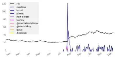
Figure 1: Example of causal features for Face-book’s stock change in 2013. The causal features (e.g., martino, k-rod) rise before the Facebook’s rapid stock rise in August.
of locally coherent pairs can suggest overall cau-sation.
In this paper, we view causality as (common-sense) cause-effect expressions that occur fre-quently in online text such as news articles or tweets. For example, “greenhouse gases causes global warming” is a sentence that provides an ‘atomic’ link that can be used in a larger chain. By connecting such causal facts in a sequence, the result can be regarded as acausal explanation be-tween the two ends of the sequence (see Table1 for examples).
This paper makes the following contributions:
• we define the problem of causal explanation generation,
• we detect causal features of a time series event (CSPIKES) using Granger (Granger, 1988) method with features extracted from text such as N-grams, topics, sentiments, and their com-position,
• we produce a large graph called CGRAPHof lo-cal cause-effect units derived from text and de-velop a method to produce causal explanations by selecting and linking appropriate units, using neural representations to enable unit matching and chaining.
[image:1.595.316.516.220.320.2]Table 1: Examples of generated causal expla-nation between some temporal causes and target companies’ stock prices.
party7−−→cut budget cuts7−−−−→lower budget bill7−−−−−→decreas republi-cans7−−−→caus obama7−−−−→leadto facebook polls7−−−→caus facebook’s stock↓
The problem of causal explanation generation arises for systems that seek to determine causal factors for events of interest automatically. For given time series events such as companies’ stock market prices, our system called CSPIKESdetects events that are deemed causally related by time series analysis using Granger Causality regres-sion (Granger,1988). We consider a large amount of text and tweets related to each company, and produces for each company time series of values for hundreds of thousands of word n-grams, topic labels, sentiment values, etc. Figure 1 shows an example of causal features that temporally causes Facebook’s stock rise in August.
However, it is difficult to understand how the statistically verified factors actually cause the changes, and whether there is a latent causal struc-ture relating the two. This paper addresses the challenge of finding such latent causal structures, in the form ofcausal explanationsthat connect the given cause-effect pair. Table 1 shows example causal explanation that our system found between
partyandFacebook’s stock fall (↓).
To construct a general causal graph, we extract all potential causal expressions from a large cor-pus of text. We refer to this graph as CGRAPH. We use FrameNet (Baker et al., 1998) semantics to provide various causative expressions (verbs, relations, and patterns), which we apply to a resource of 183,253,995 sentences of text and tweets. These expressions are considerably richer than previous rule-based patterns (Riaz and Girju, 2013; Kozareva, 2012). CGRAPH contains 5,025,636 causal edges.
Our experiment demonstrates that our causal-ity detection algorithm outperforms other baseline methods for forecasting future time series values. Also, we tested the neural reasoner on the infer-ence generation task using the BLEU score. Addi-tionally, our human evaluation shows the relative effectiveness of neural reasoners in generating ap-propriate lexicons in explanations.
2 CSPIKES: Temporal Causality Detection from Textual Features
The objective of our model is, given a target time series y, to find the best set of textual features
F = {f1, ..., fk} ⊆ X, that maximizes sum of causality over the features on y, where X is the set of all features. Note that each feature is itself a time series:
arg max
F C(y,Φ(X, y)) (1)
where C(y, x) is a causality value function be-tweenyandx, andΦis a linear composition func-tion of featuresf. Φneeds target time seriesy as well because of our graph based feature selection algorithm described in the next sections.
We first introduce the basic principles of Granger causality in Section2.1. Section 2.2 de-scribes how to extract good source featuresF =
{f1, ..., fk} from text. Section 2.3 describes the causality functionCand the feature composition functionΦ.
2.1 Granger Causality
The essential assumption behind Granger causal-ity is that a cause must occur before its effect, and can be used to predict the effect. Granger showed that given a target time series y (effect) and a source time seriesx(cause),forecastingfuture tar-get valueytwith both past target and past source time seriesE(yt|y<t, x<t)is significantly power-ful than with only past target time seriesE(yt|y<t) (plain auto-regression), if x and y are indeed a cause-effect pair. First, we learn the parameters
αandβto maximize the prediction expectation:
E(yt|y<t, xt−l) =
m X
j=1
αjyt−j+ n X
i=1
βixt−i (2)
where iand j are size of lags in the past obser-vation. Given a pair of causes x and a target y, ifβ has magnitude significantly higher than zero (according to a confidence threshold), we can say thatxcausesy.
2.2 Feature Extraction from Text
asImmigration,Syriaetc. To extract such “good” features crawled from on-line media data, we pro-pose three different types of features: Fwords,
Ftopic, andFsenti.
Fwords is time series of N-gram words that re-flect popularity of the word over time in on-line media. For each word, the number of items (e.g., tweets, blogs and news) that contains the N-gram word is counted to get the day-by-day time series. For example, xMichael Jordan = [12,51, ..] is a time series for a bi-gram word Michael Jordan. We filter out stationary words by using simple measures to estimate how dynamically the time se-ries of each word changes over time. Some of the simple measures include Shannon entropy, mean, standard deviation, maximum slope, and number of rise and fall peaks.
Ftopic is time series of latent topics with re-spect to the target time series. The latent topic is a group of semantically similar words as identi-fied by a standard topic clustering method such as LDA (Blei et al.,2003). To obtain temporal trend of the latent topics, we choose the top ten frequent words in each topic and count their occurrence in the text to get the day-by-day time series. For ex-ample, xhealthcare means how popular the topic
healthcare that consists ofinsurance,obamacare
etc, is through time.
Fsenti is time series of sentiments (positive or negative) for each topic. The top ten frequent words in each topic are used as the keywords, and tweets, blogs and news that contain at least one of these keywords are chosen to calculate the senti-ment score. The day-by-day sentisenti-ment series are then obtained by counting positive and negative words using OpinionFinder (Wilson et al.,2005), and normalized by the total number of the items that day.
2.3 Temporal Causality Detection
We define a causality function C for calculating causality score between target time series y and source time series x. The causality function C
uses Granger causality (Granger, 1988) by fitting the two time series with a Vector AutoRegressive model with exogenous variables (VARX) ( Hamil-ton, 1994): yt = αyt−l +βxt−l +t where t is a white Gaussian random vector at time t and
l is a lag term. In our problem, the number of source time series x is not single so the predic-tion happens in the kmulti-variate featuresX =
(f1, ...fk)so:
yt=αyt−l+β(f1,t−l+...+fk,t−l) +t (3)
whereαandβis the coefficient matrix of the tar-get y and source X time series respectively, and
is a residual (prediction error) for each time se-ries.βmeans contributions of each lagged feature
fk,t−lto the predicted valueyt. If the variance of
βkis reduced by the inclusion of the feature terms fk,t−l ∈ X, then it is said that fk,t−l Granger-causesy.
Our causality function C is then C(y, f, l) = ∆(βy,f,l) where ∆ is change of variance by the feature f with lagl. The total Granger causality of targetyis computed by summing the change of variance over all lags and all features:
C(y, X) =X k,l
C(y, fk, l) (4)
We compose best set of features Φ by choos-ing topkfeatures with highest causality scores for each targety. In practice, due to large amount of computation for pairwise Granger calculation, we make a bipartite graph between features and tar-gets, and address two practical problems: noisi-nessandhidden edges. We filter out noisy edges based on TFIDF and fill out missing values using non-negative matrix factorization (NMF) (Hoyer, 2004).
3 CGRAPHConstruction
Formally, given sourcex and targetyevents that are causally related in time series, if we could find a sequence of cause-effect pairs(x 7→e1),(e1 7→ e2), ... (et 7→y), thene1 7→e2, ...7→etmight be a good causal explanation betweenxandy. Sec-tion3and4describe how to bridge the causal gap between given events (x,y) by (1) constructing a large general cause-effect graph (CGRAPH) from text, (2) linking the given events to their equivalent entities in the causal graph by finding the internal paths (x 7→ e1, ...et 7→ y) as causal explanations, using neural algorithms.
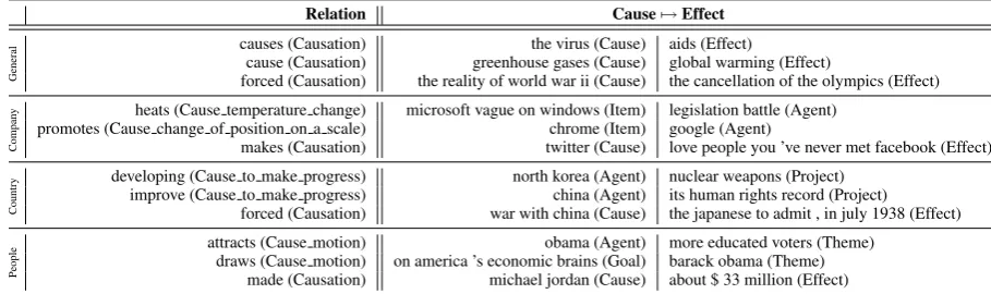
Table 2: Example (relation, cause, effect) tuples in different categories (manually labeled): general,
company,country, andpeople. FrameNet labels related to causation are listed inside parentheses. The number of distinct relation types are 892.
Relation Cause7→Effect
General
causes (Causation) the virus (Cause) aids (Effect)
cause (Causation) greenhouse gases (Cause) global warming (Effect)
forced (Causation) the reality of world war ii (Cause) the cancellation of the olympics (Effect)
Compan
y heats (Cause temperature change) microsoft vague on windows (Item) legislation battle (Agent)
promotes (Cause change of position on a scale) chrome (Item) google (Agent)
makes (Causation) twitter (Cause) love people you ’ve never met facebook (Effect)
Country
developing (Cause to make progress) north korea (Agent) nuclear weapons (Project) improve (Cause to make progress) china (Agent) its human rights record (Project)
forced (Causation) war with china (Cause) the japanese to admit , in july 1938 (Effect)
People
attracts (Cause motion) obama (Agent) more educated voters (Theme) draws (Cause motion) on america ’s economic brains (Goal) barack obama (Theme)
made (Causation) michael jordan (Cause) about $ 33 million (Effect)
as SEMAFOR (Chen et al., 2010) that produces a FrameNet style analysis of semantic predicate-argument structures, we could obtain lexical tu-ples of causation in the sentence. Since our goal is to collect only causal relations, we extract total 36 causation related frames1from the parsed sen-tences.
Table 3: Number of sentences parsed, number of entities and tuples, and number of edges (KB-KB,
KBcross) expanded by Freebase in CGRAPH.
# Sentences # Entities # Tuples #KB-KB #KBcross
183,253,995 5,623,924 5,025,636 470,250 151,752
To generate meaningful explanations, high cov-erage of the knowledge is necessary. We collect six years of tweets and NYT news articles from 1989 to 2007 (See Experiment section for details). In total, our corpus has 1.5 billion tweets and 11 million sentences from news articles. The Table3 has the number of sentences processed and num-ber of entities, relations, and tuples in the final CGRAPH.
Since the tuples extracted from text are very noisy 2, we constructed a large causal graph by linking the tuples with string match and filter out the noisy nodes and edges based on some graph statistics. We filter out nodes with very high de-gree that are mostly stop-words or auto-generated sentences. Too long or short sentences are also fil-tered out. Table2shows the (case, relation, effect) tuples with manually annotated categories such as
General,Company,Country, andPeople.
1Causation, Cause change, Causation scenario, Cause benefit or detriment, Cause bodily experience, etc.
2SEMAFOR has around62%of accuracy on held-out set.
4 Causal Reasoning
To generate a causal explanation using CGRAPH, we need traversing the graph for finding the path between given source and target events. This section describes how to efficiently traverse the graph by expanding entities with external knowl-edge base and how to find (or generate) appropri-ate causal paths to suggest an explanation using symbolic and neural reasoning algorithms. 4.1 Entity Expansion with Knowledge Base A simple choice for traversing a graph are the traditional graph searching algorithms such as Breadth-First Search (BFS). However, the graph searching procedure is likely to be incomplete (low recall), because simple string match is in-sufficient to match an effect to all its related en-tities, as it misses out in the case where an entity is semantically related but has a lexically different name.
To address thelow recallproblem and generate better explanations, we propose the use of knowl-edge base to augment our text-based causal graph with real-world semantic knowledge. We use Freebase (Google, 2016) as the external knowl-edge base for this purpose. Among 1.9 billion edges in original Freebase dump, we collect its first and second hop neighbours for each target events.
While our CGRAPH is lexical in nature, Free-base entities appear as identifiers (MIDs). For en-tity linking between two knowledge graphs, we need to annotate Freebase entities with their lex-ical names by looking at the wiki URLs. We re-fer to the edges with freebase expansion asKB-KB
[image:4.595.68.523.114.249.2]us-ing lexical matchus-ing, referrus-ing as KBcrossedges (See Table3for the number of the edges).
4.2 Symbolic Reasoning
Simple traversal algorithms such as BFS are infea-sible for traversing the CGRAPH due to the large number of nodes and edges. To reduce the search spacekinet 7→ {e1t+1, ...ekt+1}, we restricted our search by depth of paths, length of words in en-tity’s name, and edge weight.
Algorithm 1Backward Causal Inference.yis tar-get event,dis depth of BFS,lis lag size,BF Sback is Breadth-First search for one depth in backward direction, andPlCis sum of Granger causality over the lags.
1: S←y,d= 0
2: while(S=∅) or (d > Dmax)do 3: {e1−d, ...ek−d} ←BF Sback(S) 4: d=d+ 1,S←∅
5: forj in {1, ..., k}do
6: ifPlC(y, ej−d, l)< thenS←ej−d
For more efficient inference, we propose a back-ward algorithm that searches potential causes (in-stead of effects){e1
t, ...ekt} ←[ et+1 starting from the target nodey=et+1using Breadth-first search (BFS). It keeps searching backward until the node
eji has less Granger confident causality with the target nodey(See Algorithm4for causality calcu-lation). This is only possible because our system has temporal causality measure between two time series events. See Algorithm1for detail.
4.3 Neural Reasoning
While symbolic inference is fast and straightfor-ward, the sparsity of edges may make our infer-ence semantically poor. To address the lexical sparseness, we propose a lexically relaxed reason-ing usreason-ing a neural network.
Inspired by recent success on alignment task such as machine translation (Bahdanau et al., 2014), our model learns the causal alignment be-tween cause phrase and effect phrase for each type of relation between them. Rather than traversing the CGRAPH, our neural reasoner uses CGRAPH as a training resource. The encoder, a recurrent neural network such as LSTM ( Hochre-iter and Schmidhuber, 1997), takes the causal phrase while the decoder, another LSTM, takes the effectual phrase with their relation specific atten-tion.
[image:5.595.313.522.68.137.2]A submarine driver Soviet nuclear secrets
Figure 2: Our neural reasoner. The encoder takes causal phrases and decoder takes effect phrases by learning the causal alignment between them. The MLP layer in the middle takes different types of FrameNet relation and locally attend the cause to the effect w.r.t the relation (e.g., “because of”, “led to”, etc).
In original attention model (Bahdanau et al., 2014), the contextual vectorcis computed byci =
aij∗hjwherehjis hidden state of causal sequence at time j andaij is soft attention weight, trained by feed forward networkaij =F F(hj, si−1) be-tween input hidden state hj and output hidden state si−1. The global attention matrix a, how-ever, is easy to mix up all local alignment patterns of each relation.
For example, a tuple, (north korea (Agent)
developing
7−−−−−−−−−−−−−−−−−→
(Cause to make progress) nuclear weapons (Project)), is different with another tuple, (chrome (Item)
promotes
7−−−−−−−−−−−−−−−−−−→
(Cause change of position) google (Agent)) in terms of local type of causality. To deal with the local attention, we decomposed the attention weightaij by relation specific transformation in feed forward network:
aij =F F(hj, si−1, r)
whereF F has relation specific hidden layer and
r ∈ R is a type of relation in the distinct set of relationsRin training corpus (See Figure2).
Since training only with our causal graph may not be rich enough for dealing various lexical variation in text, we use pre-trained word em-bedding such as word2vec (Mikolov and Dean, 2013) trained on GoogleNews corpus3 for initial-ization. For example, given a cause phraseweapon equipped, our model could generate multiple ef-fect phrases with their likelihood: (7−−−→result
0.54 war),
(7−−−→force
0.12 army reorganized), etc, even though there are no tuples exactly matched in CGRAPH.
Table 4: Examples ofFwordswith their temporal dynamics: Shannon entropy, mean, standard devi-ation, slope of peak, and number of peaks.
entropy mean STD max slope #-peaks #lukewilliamss 0.72 22.01 18.12 6.12 31 happy thanksgiving 0.40 61.24 945.95 3423.75 414
michael jackson 0.46 141.93 701.97 389.19 585
We trained our neural reasoner in either forward or backward direction. In prediction, decoder in-ferences by predicting effect (or cause) phrase in forward (or backward) direction. As described in the Algorithm1, the backward inference continue predicting the previous causal phrases until it has high enough Granger confidence with the target event.
5 Experiment
Data. We collect on-line social media from tweets, news articles, and blogs. Our Twitter data has one million tweets per day from 2008 to 2013 that are crawled using Twitter’s Garden Hose API. News and Blog dataset have been crawled from 2010 to 2013 using Google’s news API. For target time series, we collect companies’ stock prices in NASDAQ and NYSE from 2001 until present for 6,200 companies. For presidential election polls, we collect polling data of the 2012 presidential election from 6 different websites, including USA Today , Huffington Post, Reuters, etc.
Features. For N-gram word featuresFword,we choose the spiking words based on their temporal dynamics (See Table 4). For example, if a word is too frequent or the time series is too burst, the word should be filtered out because the trend is too general to be an event. We choose five types of temporal dynamics: Shannon entropy, mean, stan-dard deviation, maximum slope of peak, and num-ber of peaks; and delete words that have too low or high entropy, too low mean and deviation, or the number of peaks and its slope is less than a certain threshold. Also, we filter out words whose frequency is less than five. From the 1,677,583 original words, we retain 21,120 words as final candidates forFwords including uni-gram and bi-gram words.
For sentiment Fsenti and topic Ftopic features, we choose 50 topics generated for both politicians and companies separately using LDA, and then use top 10 words for each topic to calculate
sen-(a)y←−−−−lag=3 rf1, ..., rfk
(b)y−−−−→lag=3 rf1, ..., rfk
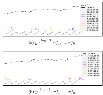
Figure 3: Random causality analysis on Googles’s stock price change (y) and randomly generated features (rf) during 2013-01-01 to 2013-12-31. (a) shows how the random features
rfcause the targety, while (b) shows how the tar-getycauses the random featuresrf with lag size of 3 days. The color changes according to causal-ity confidence to the target (blue is the strongest, and yellow is the weakest). The target time series has y scale of prices, while random features have y scale of causality degreeC(y, rf)⊂[0,1].
timent score for this topic. Then we can analyze the causality between sentiment series of a specific topic and collected time series.
Tasks. To show validity of causality detector, first we conduct random analysis between target time series and randomly generated time series. Then, we tested forecasting stock prices and elec-tion poll values with or without the detected tex-tual features to check effectiveness of our causal features. We evaluate our reasoning algorithm for generation ability compared to held-out cause-effect tuples using BLEU metric. Then, for some companies’ time series, we describe some qual-itative result of some interesting causal text fea-tures found with Granger causation and explana-tions generated by our reasoners between the tar-get and the causal features. We also conducted hu-man evaluation on the explanations.
5.1 Random Causality Analysis
To check whether our causality scoring function
regu-larly move window size of 30 over the time and generate five days of time series with a random peak strength using a SpikeM model (Matsubara et al.,2012)4. The color of random time seriesrf changes from blue to yellow according to causal-ity degree with the targetC(y, rf). For example, blue is the strongest causality with target time se-ries, while yellow is the weakest.
We observe that the strong causal (blue) features are detected just before (or after) the rapid rise of Google’ stock price on middle October in (a) (or in (b)). With the lag size of three days, we observe that the strength of the random time series gradu-ally decreases as it grows apart from the peak of target event. The random analysis shows that our causality functionCappropriately finds cause or effect relation between two time series in regard of their strength and distance.
5.2 Forecasting with Textual Features
Table 5: Forecasting errors (RMSE) on Stock andPoll data with time series only (SpikeM and
LSTM) and with time series plus text feature ( ran-dom,words,topics,sentiment, andcomposition).
Time Series Time Series + Text
Step SpikeM LSTM Crand Cwords Ctopics Csenti Ccomp
Stock
1 102.13 6.80 3.63 2.97 3.01 3.34 1.96 3 99.8 7.51 4.47 4.22 4.65 4.87 3.78 5 97.99 7.79 5.32 5.25 5.44 5.95 5.28
Poll
1 10.13 1.46 1.52 1.27 1.59 2.09 1.11 3 10.63 1.89 1.84 1.56 1.88 1.94 1.49 5 11.13 2.04 2.15 1.84 1.88 1.96 1.82
We use time series forecasting task as an eval-uation metric of whether our textual features are appropriately causing the target time series or not. Our feature composition functionΦis used to ex-tract good causal features for forecasting. We test forecasting on stock price of companies (Stock) and predicting poll value for presidential election (Poll). For stock data, We collect daily closing stock prices during 2013 for ten IT companies5. For poll data, we choose ten candidate politicians6 in the period of presidential election in 2012.
For each of stock and poll data, the future trend of target is predicted only with target’s past time
4SpikeM has specific parameters for modeling a time se-ries such as peak strength, length, etc.
5Company symbols used: TSLA, MSFT, GOOGL, YHOO, FB, IBM, ORCL, AMZN, AAPL and HPO
6Name of politicians used: Santorum, Romney, Pual, Perry, Obama, Huntsman, Gingrich, Cain, Bachmann
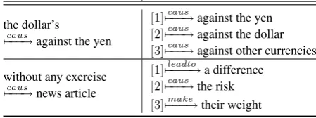
Table 6: Beam search results in neural reason-ing. These examples could be filtered out by graph heuristics before generating final explana-tion though.
Cause7→Effect in CGRAPH Beam Predictions the dollar’s
caus
7−−−→against the yen
[1]7−−−→caus against the yen
[2]7−−−→caus against the dollar
[3]7−−−→caus against other currencies without any exercise
caus
7−−−→news article
[1]7−−−−→leadto a difference
[2]7−−−→caus the risk
[3]7−−−→make their weight
series or with target’s past time series and past time series of textual features found by our system. Forecasting only with target’s past time series uses
SpikeM(Matsubara et al.,2012) that models a time series with small number of parameters and simple
LSTM (Hochreiter and Schmidhuber, 1997; nne, 2015) based time series model. Forecasting with target and textual features’ time series use Vector AutoRegressive model with exogenous variables (VARX) (Hamilton,1994) from different compo-sition function such asCrandom,Cwords,Ctopics,
Csenti, andCcomposition. Each composition func-tion exceptCrandom uses top ten textual features that causes each target time series. We also tested LSTM with past time series and textual features but VARX outperforms LSTM.
Table5shows root mean square error (RMSE) for forecasting with different step size (time steps to predict), different set of features, and different regression algorithms on stock and poll data. The forecasting error is summation of errors over mov-ing a window (30 days) by 10 days over the period. Our Ccomposition method outperforms other time series only models and time series plus text mod-els in both stock and poll data.
5.3 Generating Causality with Neural Reasoner
[image:7.595.305.530.140.224.2] [image:7.595.71.303.412.504.2]Table 7: BLEU ranking. Additional word rep-resentation +WEand relation specific alignment +REL help the model learn the cause and effect generation task especially for diverse patterns.
B@1 B@3A B@5A
S2S 10.15 8.80 8.69
S2S + WE 11.86 10.78 10.04 S2S + WE + REL 12.42 12.28 11.53
predicted phrases by beam search. For example,
B@kmeans BLEU scores for generatingk num-ber of sentences andB@kAmeans the average of them.
Table 6 shows some examples of our beam search results whenk = 3. Given a cause phrase, the neural reasoner sometime predicts semanti-cally similar phrases (e.g.,against the yen,against the dollar), while it sometimes predicts very di-verse phrases (e.g.,a different,the risk).
Table 7shows BLEU ranking results with dif-ferent reasoning algorithms: S2S is a sequence to sequence learning trained on CGRAPH by de-fault, S2S+WE adds word embedding initializa-tion, andS2S+REL+WEadds relation specific at-tention. Initializing with pre-trained word embed-dings (+WE) helps us improve on prediction. Our relation specific attention model outperforms the others, indicating that different type of relations have different alignment patterns.
5.4 Generating Explanation by Connecting Evaluating whether a sequence of phrases is rea-sonable as an explanation is very challenging task. Unfortunately, due to lack of quantitative evalua-tion measures for the task, we conduct a human annotation experiment.
Table8shows example causal chains for the rise (↑) and fall (↓) of companies’ stock price, contin-uously produced by two reasoners: SYBMis sym-bolic reasoner andNEURis neural reasoner.
We also conduct a human assessment on the ex-planation chains produced by the two reasoners, asking people to choose more convincing expla-nation chains for each feature-target pair. Table9 shows their relative preferences.
6 Related Work
Prior works on causality detection (Acharya, 2014;Anand,2014;Qiu et al.,2012) in time series
data (e.g., gene sequence, stock prices, tempera-ture) mainly use Granger (Granger, 1988) ability for predicting future values of a time series us-ing past values of its own and another time series. (Hlav´aˇckov´a-Schindler et al.,2007) studies more theoretical investigation for measuring causal in-fluence in multivariate time series based on the entropy and mutual information estimation. How-ever, none of them attempts generating explana-tion on the temporal causality.
Previous works on text causality detection use syntactic patterns such as X 7−−→verb Y, where the
verb is causative (Girju, 2003; Riaz and Girju, 2013;Kozareva, 2012; Do et al., 2011) with ad-ditional features (Blanco et al.,2008). (Kozareva, 2012) extracted cause-effect relations, where the pattern for bootstrapping has a form ofX∗ 7−−→verb
Z∗
Y from which termsX∗andZ∗was learned. The
syntax based approaches, however, are not robust to semantic variation.
As a part of SemEval (Girju et al.,2007), (Mirza and Tonelli, 2016) also uses syntactic causative patterns (Mirza and Tonelli,2014) and supervised classifier to achieve the state-of-the-art perfor-mance. Extracting the cause-effect tuples with such syntactic features or temporality (Bethard et al., 2008) would be our next step for better causal graph construction.
(Grivaz, 2010) conducts very insightful anno-tation study of what features are used in human reasoning on causation. Beyond the linguistic tests and causal chains for explaining causality in our work, other features such as counterfactuality, temporal order, and ontological asymmetry remain as our future direction to study.
Table 8: Example causal chains for explaining the rise (↑) and fall (↓) of companies’ stock price. The temporally causal featureand targetare linked through a sequence of predicted cause-effect tuples by different reasoning algorithms: a symbolic graph traverse algorithm SYMB and a neural causality reasoning modelNEUR.
SYMB
medals7−−−−→match gold and silver medals7−−−→swept korea7−−−−−−→improving relations7−−−−−→widened gap7−−−−→widens facebook↑
excess7−−−−→matchexcess materialism7−−−→causepeople make films7−−−→makemoney7−−−−−→changed twitter7−−−−→turnedfacebook↓
clinton7−−−−→matchpresident clinton7−−−−→raisedantitrust case7−−−−→matchgovernment’s antitrust case against microsoft7−−−−→matchmicrosoft7−−−→beatsapple↓
NEUR
google7−−−→forc microsoft to buy computer company dell announces recall of batteries7−−−→cause microsoft↑
the deal7−−−→make money7−−→rais at warner music and google with protest videos things7−−−→caus google↓
party7−−→cut budget cuts7−−−→lower budget bill7−−−−→decreas republicans7−−−→caus obama7−−−−→leadto facebook polls7−−−→caus facebook↓
company7−−−→forc to stock price7−−−−→leadto investors7−−−−→increas oracle s stock7−−−−→increas oracle↑
Table 9: Human evaluation on explanation chains generated by symbolic and neural reasoners.
Reasoners SYMB NEUR Accuracy (%) 42.5 57.5
function uses heuristic filters and is not robust to lexical variation.
7 Conclusion
This paper defines the novel task of detecting and explaining causes from text for a time series. First, we detect causal features from online text. Then, we construct a large cause-effect graph us-ing FrameNet semantics. By trainus-ing our relation specific neural network on paths from this graph, our model generates causality with richer lexical variation. We could produce a chain of cause and effect pairs as an explanation which shows some appropriateness. Incorporating aspects such as time, location and other event properties remains a point for future work. In our following work, we collect a sequence of causal chains verified by domain experts for more solid evaluation of gen-erating explanations.
References
2015. Neural network architecture for time series forecasting. https://github.com/hawk31/ nnet-ts.
Saurav Acharya. 2014. Causal modeling and predic-tion over event streams.
Surya Pratap Singh Tanwar Anand, Mehndiratta. 2014. Web Metric Summarization using Causal Relation-ship Graph.
Dzmitry Bahdanau, Kyunghyun Cho, and Yoshua Ben-gio. 2014. Neural machine translation by jointly learning to align and translate. arXiv preprint
arXiv:1409.0473.
Collin F Baker, Charles J Fillmore, and John B Lowe. 1998. The berkeley framenet project. In Proceed-ings of the 36th Annual Meeting of the Associa-tion for ComputaAssocia-tional Linguistics and 17th Inter-national Conference on Computational
Linguistics-Volume 1, pages 86–90. Association for
Computa-tional Linguistics.
Steven Bethard, William J Corvey, Sara Klingenstein, and James H Martin. 2008. Building a corpus of temporal-causal structure. InLREC.
Eduardo Blanco, Nuria Castell, and Dan I Moldovan. 2008. Causal relation extraction. InLREC.
David M Blei, Andrew Y Ng, and Michael I Jordan. 2003. Latent dirichlet allocation. JMLR.
Samuel R Bowman, Gabor Angeli, Christopher Potts, and Christopher D Manning. 2015. A large anno-tated corpus for learning natural language inference.
arXiv preprint arXiv:1508.05326.
Desai Chen, Nathan Schneider, Dipanjan Das, and Noah A Smith. 2010. Semafor: Frame argument resolution with log-linear models. InProceedings of the 5th international workshop on semantic evalua-tion, pages 264–267. Association for Computational Linguistics.
Qian Chen, Xiaodan Zhu, Zhenhua Ling, Si Wei, and Hui Jiang. 2016. Enhancing and combining sequen-tial and tree lstm for natural language inference.
arXiv preprint arXiv:1609.06038.
Ido Dagan, Oren Glickman, and Bernardo Magnini. 2006. The pascal recognising textual entailment challenge. In Machine learning challenges. evalu-ating predictive uncertainty, visual object
classifica-tion, and recognising tectual entailment, pages 177–
Quang Xuan Do, Yee Seng Chan, and Dan Roth. 2011. Minimally supervised event causality iden-tification. InProceedings of the Conference on
Em-pirical Methods in Natural Language Processing,
pages 294–303. Association for Computational Lin-guistics.
Roxana Girju. 2003. Automatic detection of causal re-lations for question answering. In Proceedings of the ACL 2003 workshop on Multilingual
summariza-tion and quessummariza-tion answering-Volume 12, pages 76–
83. Association for Computational Linguistics.
Roxana Girju, Preslav Nakov, Vivi Nastase, Stan Sz-pakowicz, Peter Turney, and Deniz Yuret. 2007. Semeval-2007 task 04: Classification of semantic re-lations between nominals. InProceedings of the 4th
International Workshop on Semantic Evaluations,
pages 13–18. Association for Computational Lin-guistics.
Google. 2016. Freebase Data Dumps. https: //developers.google.com/freebase/ data.
Clive WJ Granger. 1988. Some recent development in a concept of causality. Journal of econometrics, 39(1):199–211.
C´ecile Grivaz. 2010. Human judgements on causation in french texts. InLREC.
James Douglas Hamilton. 1994. Time series analysis, volume 2. Princeton university press Princeton.
Chikara Hashimoto, Kentaro Torisawa, Julien Kloetzer, and Jong-Hoon Oh. 2015. Generating event causal-ity hypotheses through semantic relations. InAAAI, pages 2396–2403.
Chikara Hashimoto, Kentaro Torisawa, Julien Kloetzer, Motoki Sano, Istv´an Varga, Jong-Hoon Oh, and Yu-taka Kidawara. 2014. Toward future scenario gener-ation: Extracting event causality exploiting semantic relation, context, and association features. InACL (1), pages 987–997.
Katerina Hlav´aˇckov´a-Schindler, Milan Paluˇs, Martin Vejmelka, and Joydeep Bhattacharya. 2007. Causal-ity detection based on information-theoretic ap-proaches in time series analysis. Physics Reports, 441(1):1–46.
Sepp Hochreiter and J¨urgen Schmidhuber. 1997. Long short-term memory. Neural computation, 9(8):1735–1780.
Patrik O Hoyer. 2004. Non-negative matrix factoriza-tion with sparseness constraints. Journal of machine
learning research, 5(Nov):1457–1469.
Vladyslav Kolesnyk, Tim Rockt¨aschel, and Sebastian Riedel. 2016. Generating natural language inference chains. arXiv preprint arXiv:1606.01404.
Zornitsa Kozareva. 2012. Cause-effect relation learn-ing. InWorkshop Proceedings of TextGraphs-7 on Graph-based Methods for Natural Language
Pro-cessing, pages 39–43. Association for
Computa-tional Linguistics.
Yasuko Matsubara, Yasushi Sakurai, B. Aditya Prakash, Lei Li, and Christos Faloutsos. 2012. Rise and fall patterns of information diffusion: model and implications. InKDD, pages 6–14.
T Mikolov and J Dean. 2013. Distributed representa-tions of words and phrases and their
compositional-ity. Advances in neural information processing
sys-tems.
Paramita Mirza and Sara Tonelli. 2014. An analysis of causality between events and its relation to temporal information. InCOLING, pages 2097–2106. Paramita Mirza and Sara Tonelli. 2016. Catena: Causal
and temporal relation extraction from natural lan-guage texts. InThe 26th International Conference
on Computational Linguistics, pages 64–75.
Kishore Papineni, Salim Roukos, Todd Ward, and Wei-Jing Zhu. 2002. Bleu: a method for automatic eval-uation of machine translation. In Proceedings of the 40th annual meeting on association for
compu-tational linguistics, pages 311–318. Association for
Computational Linguistics.
Ankur P Parikh, Oscar T¨ackstr¨om, Dipanjan Das, and Jakob Uszkoreit. 2016. A decomposable attention model for natural language inference. arXiv preprint
arXiv:1606.01933.
Huida Qiu, Yan Liu, Niranjan A Subrahmanya, and Weichang Li. 2012. Granger causality for time-series anomaly detection. InData Mining (ICDM),
2012 IEEE 12th International Conference on, pages
1074–1079. IEEE.
Mehwish Riaz and Roxana Girju. 2013. Toward a better understanding of causality between verbal events: Extraction and analysis of the causal power of verb-verb associations. InProceedings of the an-nual SIGdial Meeting on Discourse and Dialogue
(SIGDIAL). Citeseer.
Tim Rockt¨aschel, Edward Grefenstette, Karl Moritz Hermann, Tom´aˇs Koˇcisk`y, and Phil Blunsom. 2015. Reasoning about entailment with neural attention.
arXiv preprint arXiv:1509.06664.
Rebecca Sharp, Mihai Surdeanu, Peter Jansen, Pe-ter Clark, and Michael Hammond. 2016. Creating causal embeddings for question answering with min-imal supervision. arXiv preprint arXiv:1609.08097. Theresa Wilson, Janyce Wiebe, and Paul Hoffmann. 2005. Recognizing contextual polarity in phrase-level sentiment analysis. InProceedings of the con-ference on human language technology and
empiri-cal methods in natural language processing, pages