Separating Disambiguation from Composition
in Distributional Semantics
Dimitri Kartsaklis University of Oxford Dept of Computer Science Wolfson Bldg, Parks Road Oxford, OX1 3QD, UK
Mehrnoosh Sadrzadeh Queen Mary Univ. of London School of Electr. Engineering
and Computer Science Mile End Road London, E1 4NS, UK
Stephen Pulman University of Oxford Dept of Computer Science Wolfson Bldg, Parks Road Oxford, OX1 3QD, UK
Abstract
Most compositional-distributional models of meaning are based on ambiguous vec-tor representations, where all the senses of a word are fused into the same vec-tor. This paper provides evidence that the addition of a vector disambiguation step prior to the actual composition would be beneficial to the whole process, produc-ing better composite representations. Fur-thermore, we relate this issue with the current evaluation practice, showing that disambiguation-based tasks cannot reli-ably assess the quality of composition. Us-ing a word sense disambiguation scheme based on the generic procedure of Schütze (1998), we first provide a proof of con-cept for the necessity of separating dis-ambiguation from composition. Then we demonstrate the benefits of an “unambigu-ous” system on a composition-only task. 1 Introduction
Compositional and distributional semantic mod-els seem to provide complementary solutions for solving the same problem, that of assigning a proper “meaning” to a text segment. Specifically, while compositional models deal with the recur-sive nature of the language, providing a way to address its inherent ability to create infinite sen-tences from finite resources (words), they leave words as unexplained primitives whose meanings have somehow already been set before the compo-sitional process. On the other hand, distributional models have been especially successful in provid-ing concrete representations for the meanprovid-ing of words as vectors in a vector space, created by tak-ing into account the context in which each word appears. Despite its success for smaller language units, the distributional hypothesis does not natu-rally lend itself to compounds of words. Hence these models do not canonically scale in tasks re-quiring the creation of vector representations for
text constituents larger than words, i.e. for phrases and sentences.
Given the complementary nature of those two semantic models, it is not surprising that consider-able research activity has been dedicated on com-bining them into a single framework that would benefit from the best of both worlds in a uni-fied manner: Mitchell and Lapata (2008) exper-iment with intransitive sentences, applying sim-ple compositional models based on vector ad-dition and point-wise multiplication in a disam-biguation task; Baroni and Zamparelli (2010) and Guevara (2010) use regression models in order to build vectors for adjective-noun compounds; Erk and Padó (2008) work on transitive sentences us-ing structured vector spaces; Socher et al. (2010, 2011, 2012) use neural networks to combine vec-tors following the grammatical structure; Grefen-stette and Sadrzadeh (2011a,b) apply the categori-cal framework of Coecke et al. (2010) on the dis-ambiguation task of Mitchell and Lapata (2008); and Kartsaklis et al. (2012) and Grefenstette et al. (2013) build upon previous implementations by adding specific algebraic operations and machine learning techniques to further improve the con-crete abilities of the abstract categorical models.
A common strand in all of the above models is that they are based on “ambiguous” vector rep-resentations, where a polysemous word is repre-sented by a single vector regardless of the number of its actual senses. For example, the word ‘bank’ has at least two meanings (financial institution and land alongside a river), both of which will be fused into a single vector representation. And, although it is generally true that compositional models fol-lowing the formal semantics view of Montague do not care about disambiguation (meanings of words in such models are represented by logical con-stants explicitly set before the compositional pro-cess), the story changes when one moves to a vec-tor space model with ambiguous vecvec-tor represen-tations. The main problem is that, when acting on ambiguous vector spaces, compositional models
seem to perform two tasks at the same time, com-positionanddisambiguation, leaving the resulting vector hard to interpret: it is not clear if this vector is a proper meaning representation for the com-posed compound or just a disambiguated version of one of the words therein. This problem escapes the evaluation schemes, especially when disam-biguation tasks are used as a criterion for evaluat-ing compositional models—a common practice in current research for compositional-distributional semantics. Indeed, Pulman (2013) argues that al-though disambiguation can emerge as a welcome side-effect of the compositional process, it is not clear if compositionality is either a necessary or sufficient condition for disambiguation to happen. On the contrary, it seems that the form of most current vector space models and the compositional operations used on them (quite often some form of vector point-wise multiplication) mainly achieve disambiguation, but not composition.
The purpose of this paper is to further investi-gate the potential of a compositional-distributional model based on disambiguated vector represen-tations, where each word can have one or more distinct senses. More specifically, we aim to show that (a) compositionality is not a neces-sary condition for disambiguation, so the quite common practice of using a disambiguation task as a criterion for evaluating the performance of compositional-distributional models is question-able; and (b) the introduction of a separate disam-biguation step in the compositional process of dis-tributional models can be indeed beneficial for the quality of the resulting composed vectors.
We train our models from BNC, a 100-million words corpus created from samples of written and spoken English. We perform word sense induc-tion by following the generic algorithm of Schütze (1998), in which the senses of a word are repre-sented by distinct clusters created by taking into account the various contexts in which this specific word occur in the corpus. For the actual cluster-ing step we use a combination of hierarchical ag-glomerative clustering and the Cali´nski-Harabasz index (Cali´nski and Harabasz, 1974). The param-eters of the models are fine-tuned on the noun set of SEMEVAL2010 Word Sense Induction and Dis-ambiguation task (Manandhar et al., 2010).
Equipped with a disambiguated vector space, we use it on a verb disambiguation experiment, similar in style to that of Mitchell and Lapata (2008), but applied on a more linguistically mo-tivated dataset, based on the work of Pickering and Frisson (2001). We find that the application
of a simple disambiguation algorithm,withoutany compositional steps, is proven more effective than a number of compositional models. We consider this as an indication for the necessity of separat-ing disambiguation from composition, since it im-plies that the latter is not necessary for achiev-ing the former. Next, we demonstrate that a com-positional model based on disambiguated vectors can indeed produce composite vector representa-tions of better quality, by applying the model on a phrase similarity task (Mitchell and Lapata, 2010). The goal here is to evaluate the similarity of short verb phrases, based on the distance of their com-posite vectors.
2 Composition in distributional models The transition from word meaning to sentence meaning, a task easily done by human subjects based on the rules of grammar, implies the exis-tence of a composition operation applied to prim-itive text units in order to build compound ones. Various solutions have been proposed with differ-ent levels of sophistication for this problem in the context of vector space models of meaning.
At one end of the spectrum the simple models of Mitchell and Lapata (2008) address composi-tion as the point-wise multiplicacomposi-tion or addicomposi-tion of the involved word vectors. This bag-of-words approach has been proven a hard-to-beat baseline for many of the more sophisticated models. At the other end, composition in the work of Socher et al. (2010, 2011, 2012) is served by the advanced ma-chinery of recurring neural networks, where the output of the network is used again as input in a recurring fashion, for composing vectors of larger constituents. Following a different path, the cat-egorical framework of Coecke et al. (2010) ex-ploits a structural homomorphism between gram-mar and vector spaces in order to treat words with special meanings, such as verb and adjectives, as functions (tensors of rank-n) that apply to their ar-guments. This application has the form of inner product, generalising the familiar notion of matrix multiplication to tensors of higher rank.
Regardless of their level of sophistication, most of the models which aim to apply composition-ality on word vector representations fail to ad-dress the problem of handling the polysemous na-ture of words. Even more importantly, many of the models are evaluated on their ability to
dis-ambiguatethe meaning of specific words,
au-thors test their multiplicative and additive models as follows: given an ambiguous intransitive verb, say ‘run’ (with the two senses to be those of mov-ing fast and of a liquid dissolvmov-ing), they examine to what extent the composition of the verb with an appropriate subject (e.g. ‘horse’ or ‘colour’) will disambiguate the intended sense of the verb within the specific context. Each row in the dataset consists of a subject (e.g. ‘horse’), a verb (‘run’), a high-similarity landmark verb (‘gallop’), and a low-similarity landmark verb (‘dissolve’). The subject is combined with the main verb to form a simple intransitive sentence, and the vector of this sentence is then compared with the vectors of the landmark verbs. The goal is to evaluate the degree to which the composed sentence vector is closer to the high landmark than to the vector of the low landmark, and this is considered an indication of successful composition.
However, although it is generally true that mul-tiplying−−→runwith−−−→horsewill filter out most of the components of−−→runthat are irrelevant to ‘dissolve’ (since the ‘dissolve’-related elements of −−−→horse should have values close to zero) and will pro-duce a disambiguated version of this verb under the context of ‘horse’, it is not at all clear if this vector will also constitute an appropriate repre-sentation for the meaning of the intransitive sen-tence ‘horse runs’. In other words, here we have two tasks taking place at the same time: (a) dis-ambiguation of the ambiguous word given its con-text; and (b) composition that produces a mean-ing vector for the whole sentence. The extent to which the latter is a necessary condition for the former remains unclear, and constitutes a factor that complicates the evaluation and assessment of such systems. In this paper we argue that as long as the above distinct tasks are interwoven into a single step, claims of compositionality in distri-butional systems cannot be reliably assessed. We therefore propose the addition of a disambiguation step in the generic methodology of compositional-distributional models.
3 Related work
Although in general word sense induction is a popular topic in the natural language processing literature, little has been done to address poly-semy specifically in the context of compositional-distributional models of meaning. In fact, the only works relevant to ours we are aware of are that of Erk and Padó (2008) and Reddy et al. (2011). The structured vector space of Erk and Padó (2008) is designed to handle ambiguity in an implicit way,
showing promising results on the Mitchell and Lapata (2008) task. The work of Reddy et al. (2011) is closer to our research: the authors eval-uate two word sense disambiguation approaches on the noun-noun compound similarity task intro-duced by Mitchell and Lapata (2010), using sim-ple multiplicative and additive models for compo-sition. The reported results are also promising, where at least one of their models performs bet-ter than the current practice of using ambiguous vector representations.
Compared to both of the above works, the scope of the current paper is broader: it does not solely aim to demonstrate the positive effect of a “cleaner” vector space on the compositional pro-cess, but it also proceeds one step further and re-lates this issue with the current evaluation prac-tice, showing that a number of verb disambigua-tion tasks that have been invariantly used for the assessment of compositional-distributional mod-els might be in fact based on a wrong criterion. 4 Disambiguation scheme
Our word sense induction method is based on the effective procedure first presented by Schütze (1998). For theith occurrence of a target wordwt
in the corpus with context Ci = {w1, . . . , wn},
we calculate the centroid of the context as −→ci =
1
n(−w→1 + . . . +−→wn), where −→w is the lexical (or
first order) vector of wordwas it is created by the
usual distributional practice (more details in Sec-tion 5). Then, we cluster these centroids in order to form a number of sense clusters. Each sense of the word is represented by the centroid of the corresponding cluster. Following Schütze, we will refer to these sense vectors as second-order vec-tors, in order to distinguish them from the lexical (first-order) vectors. So, in our model each word is represented by a tupleh−→w , Si, where−→w is the 1st-order vector of the word andSthe set of 2nd-order vectors created by the above procedure.
We are now able to disambiguate the sense of a target wordwtgiven a contextC by calculating a
context vector−→c forC as above, and then com-paring this with every 2nd-order vector ofwt; the
word is assigned to the sense that corresponds to the closest 2nd-order vector. That is,
−−→
spref= arg min
− →s∈S d(
−
→s ,−→c) (1)
whereSis the set of 2nd-order vectors forwtand
clus-1 0 1 2 3 4 5 1.0
0.5 0.0 0.5 1.0 1.5 2.0 2.5 3.0 3.5
23 27 28 20 29 24 22 25 21 26 14 13 16 15 11 19 17 18 10 12 8 1 3 6 9 4 2 7 0 5
[image:4.595.72.285.61.138.2]0.0 0.2 0.4 0.6 0.8 1.0 1.2 1.4
Figure 1: Hierarchical agglomerative clustering.
tering has been invariably applied to unsupervised word sense induction on a variety of languages, generally showing good performance—see, for example, the comparative study of Broda and Mazur (2012) for English and Polish. Compared tok-means clustering, this approach has the ma-jor advantage that it does not require us to define in advance a specific number of clusters. Com-pared to more advanced probabilistic techniques, such as Bayesian mixture models, it is much more straightforward and simple to implement, yet powerful enough to demonstrate the necessity of factoring out ambiguity from compositional-distributional models.
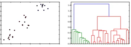
HAC is a bottom-up method of cluster analy-sis, starting with each data point (context vector in our case) forming its own cluster; then, in each it-eration the two closest clusters are merged into a new cluster, until all points are finally merged un-der the same cluster. This process produces a
den-drogram (i.e. a tree diagram), which essentially
embeds every possible clustering of the dataset. As an example, Figure 1 shows a small dataset produced by three distinct Gaussian distributions, and the dendrogram derived by the above algo-rithm. Implementation-wise, the clustering part in this work is served by the efficient FASTCLUSTER library (Müllner, 2013).
Choosing a number of senses In HAC, one still needs to decide where exactly to cut the tree in or-der to get the best possible partitioning of the data. Although the right answer to this problem might depend on many factors, we can safely assume that the optimal partitioning is the one that provides the most compact and maximally separated clus-ters. One way to measure the quality of a cluster-ing based on this criterion is the Cali´nski/Harabasz index (Cali´nski and Harabasz, 1974), also known as variance ratio criterion (VRC). Given a set ofN data points and a partitioning ofkdisjoint clusters, VRC is computed as follows:
V RCk =
trace(B) trace(W) ×
N−k
k−1 (2) Here, W andB are the intra-cluster and inter-cluster dispersion matrices, respectively:
W =
k
X
i=1
Ni
X
l=1
(→−xi(l)−x¯i)(→−xi(l)−x¯i)T (3)
B=
k
X
i=1
Ni( ¯xi−x)( ¯¯ xi−x)¯ T (4)
whereNi is the number of data points assigned to
clusteri,−→xi(l)is thelth point assigned to this
clus-ter,x¯iis the centroid ofith cluster (the mean), and
¯
xis the data centroid of the overall dataset. Given the above formulas, the trace of B is the sum of inter-cluster variances, while the trace ofW is the sum of intra-cluster variances. A good partitioning should have high values forB (which is an indi-cation for well-separated clusters) and low values forW (an indication for compact clusters), so the higher the quality of the partitioning the greater the value of this ratio.
Compared to other criteria, VRC has been found to be one of the most effective approaches for clustering validity—see the comparative stud-ies of Milligan and Cooper (1985) and Vendramin et al. (2009). Furthermore, it has been previously applied to word sense discrimination successfully, returning the best results among a number of other measures (Savova et al., 2006). For this work, we calculate VRC for a number of different partition-ings (ranged from 2 to 10 clusters), and we keep the partitioning that results in the highest VRC value as the optimal number of senses for the spe-cific word. Note that since the HAC dendrogram already embeds all possible clusterings, the cut-ting of the tree in order to get a different partition-ing is performed in constant time.
5 Experimental setting
The choice of our 1st-order vector space is based on empirical tests, where we found out that a basis with elements of the form hword,classi presents the right balance for our purposes among sim-pler techniques, such as word-based spaces, and more complex ones, such as dependency-based approaches. In our vector space, each word has a distinct vector representation for every word class under which occurs in the corpus (e.g. ‘suit’ will have a noun vector and a verb vector). As our ba-sis elements we use the 2000 most frequent con-tent words in BNC, with weights being calculated as the ratio of the probability of the context word given the target word to the probability of the con-text word overall. The concon-text here is a 5-word window on both sides of the target word.
Sense Induction & Disambiguation Task (Man-andhar et al., 2010). Specifically, when using HAC one has to decide how to measure the distance between the clusters, which is the merging crite-rion applied in every iteration of the algorithm, as well as the measure between the data points, i.e. the individual vectors. Based on empirical tests we limit our options to two inter-cluster mea-sures: complete-link and Ward’s methods. In the complete-link method the distance between two clustersXandY is the distance between their two most remote elements:
D(X, Y) = max
x∈X,y∈Y d(x, y) (5)
In Ward’s method, two clusters are selected for merging if the new partitioning exhibits the mini-mum increase in the overall intra-cluster variance. The cluster distance is given by:
D(X, Y) = 2|X||Y|
|X|+|Y|k−c→X − −c→Yk
2 (6)
where−c→X and−c→Y are the centroids ofXandY.
We test these linkage methods in combination with three vector distance measures: euclidean, cosine, and Pearson’s correlation (6 models in to-tal). The metrics were chosen to represent pro-gressively more relaxed forms of vector compar-ison, with the strictest form to be the euclidean distance and correlation as the most relaxed. For sense detection we use the disambiguation algo-rithm described in Section 4, considering as con-text the whole sentence in which a target word appears. The distance metric used for the dis-ambiguation process in each model is identical to the metric used for the clustering process, so in the Ward/euclidean model the disambiguation is based on the euclidean distance, in complete-link/cosine model on the cosine distance, and so on. We evaluate the models using V-measure, an entropy-based metric that addresses the
so-Model V-Meas. Avg clust.
Ward/Euclidean 0.05 1.44
Ward/Correlation 0.14 3.14
Ward/Cosine 0.08 1.94
Complete/Euclidean 0.00 1.00 Complete/Correlation 0.11 2.66 Complete/Cosine 0.06 1.74 Most frequent sense 0.00 1.00 1 cluster/instance 0.36 89.15
Gold standard 1.0 4.46
Table 1: Results on the noun set of SEMEVAL 2010 WSI&D task.
keyboard:1105 contexts, 2 senses
COMPUTER(665 contexts): program dollar disk power enter port graphic card option select language drive pen application corp external editor woman price page design sun cli amstrad lock interface lcd slot notebook
MUSIC (440 contexts): drummer instrumental singer
german father fantasia english generation wolfgang wayne cello body join ensemble mike chamber gary saxophone sax ricercarus apply form son metal guy clean roll barry orchestra
Table 2: Derived senses for word ‘keyboard’.
called matching problem of F-score (Rosenberg and Hirschberg, 2007). Table 1 shows the results.
Ward’s method in combination with correla-tion distance provided the highest V-measure, fol-lowed by the combination of complete-link with (again) correlation. Although a direct compari-son of our models with the models participating in this task would not be quite sound (since these models were trained on a special corpus provided by the organizers, while our model was trained on the BNC), it is nevertheless enlightening to mention that the 0.14 V-measure places the Ward-correlation model at the 4th rank among 28 sys-tems for the noun set of the task, while at the same time provides a reasonable average number of clusters per word (3.14), close to that of the human-annotated gold standard (4.46). Compare this, for example, with the best-performing sys-tem that achieved a V-measure of 0.21, a score that was largely due to the fact that the model as-signed the unrealistic number of 11.54 senses per word on average (since V-measure tends to favour higher numbers of senses, as the baseline1
clus-ter/instanceshows in Table 1).1
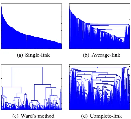
Table 2 provides an example of the results, showing the senses for the noun ‘keyboard’ learnt by the best model of Ward’s method and correla-tion measure. Each sense is visualized as a list of the most dominant words in the cluster, ranked by their TF-ICFvalues. Furthermore, Figure 2 shows the dendrograms produced by four linkage meth-ods for the word ‘keyboard’, demonstrating the su-periority of Ward’s method.
6 Disambiguation vs composition
A number of models that aim to equip distribu-tional semantics with composidistribu-tionality are evalu-ated on some form of the disambiguation task pre-sented in Section 2. Versions of this task can be found, for example, in Mitchell and Lapata (2008),
1The results of SEMEVAL2010 can be found online at http://www.cs.york.ac.uk/semeval2010_WSI/task_14
0.0 0.1 0.2 0.3 0.4 0.5 0.6
keyboard (single/cosine)
(a) Single-link 0.0
0.2 0.4 0.6 0.8
keyboard (average/cosine)
(b) Average-link
0 1 2 3 4 5
keyboard (ward/cosine)
(c) Ward’s method 0.0
0.2 0.4 0.6 0.8
1.0 keyboard (complete/cosine)
[image:6.595.72.284.57.250.2](d) Complete-link
Figure 2: Dendrograms produced for word ‘key-board’ according to 4 different linkage methods.
Erk and Padó (2008), Grefenstette and Sadrzadeh (2011a,b), Kartsaklis et al. (2012) and Grefenstette et al. (2013). We briefly remind that the goal is to assess how well a compositional model can disam-biguate the meaning of an ambiguous verb, given a specific context. This kind of evaluation involves two distinct tasks: the composition of sentence vectors, and the disambiguation of the verbs. And, although the evaluation of a model against human judgements provides some indication for the suc-cess of the latter task, it leaves unclear to what ex-tent the former has been achieved. In this section we perform two experiments in order to address this question. The first of them aims to support the following argument: that although disambiguation can emerge as a side-effect of a compositional pro-cess, compositionality is not a necessary condition for this to happen. The second experiment is based on a more appropriate task that requires genuine compositional abilities, and demonstrates the good performance of a compositional model based on the disambiguated vector space of Section 5.
As our compositional method for the follow-ing tasks we use the multiplicative and additive models of Mitchell and Lapata (2008). Despite the simple nature of these models, there is a num-ber of reasons that make them good candidates for demonstrating the main ideas of this paper. First, for better or worse “simple” does not necessar-ily mean “ineffective”. The comparative study of Blacoe and Lapata (2012) shows that for certain tasks these “baselines” perform equally well or even better than other more sophisticated models. And second, it is reasonable to expect that better compositional models would only work in favour of our arguments, and not the other way around.
6.1 Evaluating disambiguation
One potential problem with the datasets used for the disambiguation task of Section 2, similar to the one of Grefenstette and Sadrzadeh (2011a), is that ambiguous verbs are usually collected from a corpus based on some automated method. And, although they do exhibit variations in their senses (as most verbs do), in many cases these meanings are actually related—for example, the meanings of ‘write’ in G&S dataset are spellandpublish. To overcome this problem, we used the work of Pick-ering and Frisson (2001), which provides a list of genuinely ambiguous verbs obtained from careful manual selection and ranking from human evalu-ators. The evaluators assessed the relatedness of each verb’s different meanings using a scale of 0 (totally unrelated) to 7 (highly related). From these verbs, we picked 10 with an average mark <1. An example is ‘file’, which means ‘smooth’ in ‘file nails’ and ‘register’ as in ‘file an applica-tion’. For each verb we picked the 10 most oc-curring subjects and objects from the BNC (5 for each landmark). In the case of verb ‘file’, for ex-ample, among these were ‘woman’ and ‘nails’ for landmark ‘smooth’, and ‘union’ and ‘lawsuit’ for landmark ‘register’. Each subject and object was modified by its most occurring adjective in the cor-pus. This resulted in triples of sentences of the following form:
(1) main: young woman filed long nails
high: young woman smoothed long nails
low: young woman registered long nails (2) main: monetary union filed civil lawsuit
high: mon. union registered civil lawsuit
low: mon. union smoothed civil lawsuit
The main sentence was paired with both high and low landmark sentences, creating a dataset2of 200 sentence pairs (10 main verbs ×10 contexts ×2 landmarks)3. These were randomly presented to 43 human annotators, whose duty was to judge the similarity between the sentences of each pair. The human scores were compared with scores pro-duced by a number of models (Table 3).
The most successful model (M1) does not ap-ply any form of composition. Instead, the com-parison of a sentence with a “landmark” sentence is simply based on disambiguated versions of the
2The dataset will be available at http://www.cs.ox. ac.uk/activities/compdistmeaning/.
3As a comparison, the Mitchell and Lapata (2008) dataset
verbs alone. Specifically, the main verb and the landmark verb are disambiguated given the con-text (subjects, objects, and adjectives that mod-ify them) according to Equation 1; this produces two 2nd-order vectors, one for the main verb and one for the landmark. The degree of similarity be-tween the two sentences is then calculated by mea-suring the similarity between the two sense vec-tors of the verbs, without any compositional step. The score of 0.28 achieved by this model is im-pressive, given that the inter-annotator agreement (which serves as an upper-bound) is 0.38.
A number of interesting observations can be made based on the results of Table 3. First of all, the ‘verbs-only’ model outperforms the two baselines (which use composition but not disam-biguation) by a large margin, and indeed also the other compositional models. This is an indica-tion that this kind of disambiguaindica-tion task might not be the best way to evaluate a compositional model. The fact that the most important condi-tion for success is the proper disambiguacondi-tion of the verb, means that the good performance of a compositional model demonstrates only this: how well the model is able to disambiguate an am-biguous verb. This is different from how well the composed representation reflects the meaning of the larger constituent; that is, it has very little to say about the extent to which an operation like
−−−−−→
woman−−→f ile−−−→nails(denotes point-wise mul-tiplication) results in a faithful representation of the meaning of sentence ‘woman filed nails’.
M2 to M5 represent different versions of the compositional models that use disambiguation in a distinct step. All these models compose both the main verb and the landmark with a given context, and then perform the comparison at sentence level. In M2 and M3 all words are first disambiguated prior to composition, while in M4 and M5 the
2nd-Disambig. Composition ρ
M1 Only verbs No 0.282 ∗
M2 All words Multiplicative 0.118 M3 All words Additive 0.210 M4 Only verbs Multiplicative 0.110 M5 Only verbs Additive 0.234 ∗
B1 No Multiplicative 0.143
B2 No Additive 0.042
Inter-annotator agreement 0.383
∗The difference between M1 and M5 is highly
statistically significant withp <0.0001
Table 3: Spearman’sρfor the Pickering and Fris-son dataset.
order vector of the verb is composed with the 1st-order vectors of the other words. The most im-pressive observation here is that the separation of disambiguation results in a tremendous improve-ment for the additive model, from 0.04 to 0.21. This is not surprising since, when using magni-tude invariant measures between vectors (such as cosine distance), the resulting vector is nothing more than the average of the involved word vec-tors. The introduction of the disambiguation step before the composition, therefore, makes a great difference since it provides much more accurate starting points to be averaged.
On the other hand, the disambiguated version of multiplicative model (M2) presents inferior per-formance compared to the “ambiguous” version (B1). We argue that the reason behind this is that the two models perform different jobs: the result of B1 is a “mixing” of composition and disam-biguation of the most ambiguous word (i.e. the verb), since this is the natural effect of the point-wise multiplication operation (see discussion in Section 2); on the other hand, M2 is designed to construct an appropriate composite meaning for the whole sentence. We will try to support this argument by the experiment of the next section.
6.2 A better test of compositionality
Although there might not exists such a thing asthe best evaluation method for compositional-distributional semantics, it is safe to assume that a phrase similarity task avoids many of the pitfalls of tasks such as the one of Section 6.1. Given pairs of short phrases, the goal is to assess the similar-ity of the phrases by constructing composite vec-tors for them and computing their distance. No as-sumptions about disambiguation abilities regard-ing a specific word (e.g. the verb) are made here; the only criterion is to what extent the composite vector representing the meaning of a phrase is sim-ilar or dissimsim-ilar to the vector of another phrase. From this perspective, this task seems the ideal choice for evaluating a model aiming to provide appropriate phrasal semantics. The scores given by the models are compared to those of human evaluators using Spearman’sρ.
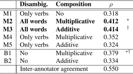
For this experiment, we use the “verb-object” part of the dataset presented in the work of Mitchell and Lapata (2010), which consists of 108 pairs of short verb phrases exhibiting three de-grees of similarity. A high similarity pair for ex-ample, isproduce effect/achieve result, a medium one ispour tea/join party, and a low one isclose
con-Disambig. Composition ρ
M1 Only verbs No 0.318
M2 All words Multiplicative 0.412 ∗ M3 All words Additive 0.414 †
M4 Only verbs Multiplicative 0.352 M5 Only verbs Additive 0.324
B1 No Multiplicative 0.379 ∗†
B2 No Additive 0.334
Inter-annotator agreement 0.550
∗Difference between M2/B1 is stat. sign. withp≤0.07
[image:8.595.73.295.63.186.2]†Difference between M3/B1 is stat. sign. withp≤0.06
Table 4: Phrase similarity results.
tains noun-noun and adjective-noun compounds. However, the verb-object part serves the pur-poses of this paper much better, for two reasons. First, since by definition the proposed methodol-ogy suits better circumstances involving at least some level of word ambiguity, a dataset based on the most ambiguous part of speech (verbs) seems a reasonable choice. Second, this part of the dataset allows us to do some meaningful comparisons with the task of Section 6.1, which is again around verb structures. The results are shown in Table 4.
This time, the disambiguation step provides solid benefits for both multiplicative (M2) and additive (M3) models, with differences that are statistically significant from the best baseline B1 (with p ≤ 0.07 and p ≤ 0.06, respectively). Note that the ‘verbs-only’ model (M1), which was by a large margin the most successful for the task of Section 6.1, now shows the worst perfor-mance. For comparison, the best result reported by Mitchell and Lapata (2010) on a 1st-order space similar to ours (regarding dimensions and weights) was 0.38 (“dilation” model).
7 Discussion
This paper is based on the observation that any compositional operation between two vectors is essentially a hybrid process consisting of two “components” that, depending on the form of the underlying vector space, can have different “mag-nitudes”. One of the components results in a cer-tain amount of disambiguation for the most am-biguous original word, while the other one works towards a composite representation for the mean-ing of the whole phrase or sentence. The tasks of Section 6 are designed so that each one of them as-sesses a different aspect of this hybrid process: the task of Section 6.1 is focused on the disambigua-tion aspect, while the task of Secdisambigua-tion 6.2 addresses the compositionality part. One of our main
argu-ments is the observation that, in order the get bet-ter compositional representations, it is essential to first eliminate (or at least reduce as much as pos-sible the magnitude of) the disambiguation “com-ponent” that might show up as a by-product of the compositional process, so that the result is mainly a product of pure composition—this is what the “unambiguous” models do achieve in the task of Section 6.2. Based on the experimental work con-ducted in this paper, our first concluding remark is that the elimination of the ambiguity factor can be essential for the quality of the composed vectors.
But, if Table 4 provides a proof that the sep-aration of disambiguation and composition can indeed produce better compositional representa-tions, what is the meaning of the inferior perfor-mance of all “unambiguous” models (M2 to M5) compared to verbs-only version (M1) in the task of Section 6.1? Why disambiguation is not always effective (as in the case of multiplicative model) for that task? These are strong indications that the quality of composition is not crucial for disam-biguation tasks of this sort, whose only achieve-ment is that they measure the disambiguation side-effects generated by the compositional process. In other words, the practice of evaluating the qual-ity of composition by using disambiguation tasks is problematic. As the topic of compositionality in distributional models of meaning increasingly gains popularity in the recent years, this second concluding remark is equally important since it can contribute towards better evaluation schemes of such models.
8 Future work
A next step to take in the future is the appli-cation of these ideas on more complex spaces, such as those based on the categorical framework of Coecke et al. (2010). The challenge here is the effective generalization of a disambiguation scheme on tensors of rank greater than 1. Ad-ditionally, we would expect this method to bene-fit from more robust probabilistic clustering tech-niques. An appealing option is the use of a non-parametric method, such as a hierarchical Dirich-let process (Yao and Van Durme, 2011).
Acknowledgements
References
Baroni, M. and Zamparelli, R. (2010). Nouns are Vectors, Adjectives are Matrices. In Pro-ceedings of Conference on Empirical Methods
in Natural Language Processing (EMNLP).
Blacoe, W. and Lapata, M. (2012). A compari-son of vector-based representations for seman-tic composition. In Proceedings of the 2012 Joint Conference on Empirical Methods in Nat-ural Language Processing and Computational
Natural Language Learning, pages 546–556,
Jeju Island, Korea. Association for Computa-tional Linguistics.
Broda, B. and Mazur, W. (2012). Evaluation of clustering algorithms for word sense disam-biguation. International Journal of Data
Anal-ysis Techniques and Strategies, 4(3):219–236.
Cali´nski, T. and Harabasz, J. (1974). A Dendrite Method for Cluster Analysis. Communications
in Statistics-Theory and Methods, 3(1):1–27.
Coecke, B., Sadrzadeh, M., and Clark, S. (2010). Mathematical Foundations for Dis-tributed Compositional Model of Meaning. Lambek Festschrift. Linguistic Analysis, 36:345–384.
Erk, K. and Padó, S. (2008). A Structured Vector-Space Model for Word Meaning in Context. In
Proceedings of Conference on Empirical
Meth-ods in Natural Language Processing (EMNLP),
pages 897–906.
Grefenstette, E., Dinu, G., Zhang, Y.-Z., Sadrzadeh, M., and Baroni, M. (2013). Multi-step regression learning for compositional dis-tributional semantics.
Grefenstette, E. and Sadrzadeh, M. (2011a). Ex-perimental Support for a Categorical Composi-tional DistribuComposi-tional Model of Meaning. In Pro-ceedings of Conference on Empirical Methods
in Natural Language Processing (EMNLP).
Grefenstette, E. and Sadrzadeh, M. (2011b). Ex-perimenting with Transitive Verbs in a DisCo-Cat. In Proceedings of Workshop on Geomet-rical Models of Natural Language Semantics
(GEMS).
Guevara, E. (2010). A Regression Model of Adjective-Noun Compositionality in Distribu-tional Semantics. In Proceedings of the ACL
GEMS Workshop.
Kartsaklis, D., Sadrzadeh, M., and Pulman, S. (2012). A unified sentence space for categorical distributional-compositional semantics: Theory
and experiments. InProceedings of 24th Inter-national Conference on Computational
Linguis-tics (COLING 2012): Posters, pages 549–558,
Mumbai, India. The COLING 2012 Organizing Committee.
Kintsch, W. (2001). Predication. Cognitive Sci-ence, 25(2):173–202.
Manandhar, S., Klapaftis, I., Dligach, D., and Pradhan, S. (2010). Semeval-2010 task 14: Word sense induction & disambiguation. In
Proceedings of the 5th International Workshop
on Semantic Evaluation, pages 63–68.
Associa-tion for ComputaAssocia-tional Linguistics.
Milligan, G. and Cooper, M. (1985). An Exami-nation of Procedures for Determining the Num-ber of Clusters in a Data Set. Psychometrika, 50(2):159–179.
Mitchell, J. and Lapata, M. (2008). Vector-based Models of Semantic Composition. In Proceed-ings of the 46th Annual Meeting of the
Associa-tion for ComputaAssocia-tional Linguistics, pages 236–
244.
Mitchell, J. and Lapata, M. (2010). Composition in distributional models of semantics.Cognitive
Science, 34(8):1388–1439.
Müllner, D. (2013). fastcluster: Fast Hierarchical Clustering Routines for R and Python. Journal
of Statistical Software, 9(53):1–18.
Pickering, M. and Frisson, S. (2001). Process-ing ambiguous verbs: Evidence from eye move-ments. Journal of Experimental Psychology:
Learning, Memory, and Cognition, 27(2):556.
Pulman, S. (2013). Combining Compositional and Distributional Models of Semantics. In Heunen, C., Sadrzadeh, M., and Grefenstette, E., editors,
Quantum Physics and Linguistics: A
Composi-tional, Diagrammatic Discourse. Oxford
Uni-versity Press.
Reddy, S., Klapaftis, I., McCarthy, D., and Man-andhar, S. (2011). Dynamic and static prototype vectors for semantic composition. In Proceed-ings of 5th International Joint Conference on
Natural Language Processing, pages 705–713.
Rosenberg, A. and Hirschberg, J. (2007). V-measure: A conditional entropy-based external cluster evaluation measure. In Proceedings of the 2007 Joint Conference on Empirical Meth-ods in Natural Language Processing and
Com-putational Natural Language Learning, pages
Savova, G., Therneau, T., and Chute, C. (2006). Cluster Stopping Rules for Word Sense Dis-crimination. In Proceedings of the workshop on Making Sense of Sense: Bringing Psy-cholinguistics and Computational Linguistics
Together, pages 9–16.
Schütze, H. (1998). Automatic Word Sense Dis-crimination.Computational Linguistics, 24:97– 123.
Socher, R., Huang, E., Pennington, J., Ng, A., and Manning, C. (2011). Dynamic Pooling and Un-folding Recursive Autoencoders for Paraphrase Detection. Advances in Neural Information
Processing Systems, 24.
Socher, R., Huval, B., Manning, C., and A., N. (2012). Semantic compositionality through re-cursive matrix-vector spaces. InConference on Empirical Methods in Natural Language
Pro-cessing 2012.
Socher, R., Manning, C., and Ng, A. (2010). Learning Continuous Pphrase Representations and Syntactic Parsing with recursive neural net-works. InProceedings of the NIPS-2010 Deep Learning and Unsupervised Feature Learning
Workshop.
Vendramin, L., Campello, R., and Hruschka, E. (2009). On the Comparison of Relative Clus-tering Validity Criteria. In Proceedings of the SIAM International Conference on Data
Min-ing, SIAM, pages 733–744.