Automatically Constructing a Normalisation Dictionary for Microblogs
Bo Han,♠♥Paul Cook,♥ and Timothy Baldwin♠♥
♠NICTA Victoria Research Laboratory
♥Department of Computing and Information Systems, The University of Melbourne
[email protected], [email protected],
Abstract
Microblog normalisation methods often utilise complex models and struggle to differenti-ate between correctly-spelled unknown words and lexical variants of known words. In this paper, we propose a method for construct-ing a dictionary of lexical variants of known words that facilitates lexical normalisation via simple string substitution (e.g.tomorrow for tmrw). We use context information to generate possible variant and normalisation pairs and then rank these by string similarity. Highly-ranked pairs are selected to populate the dic-tionary. We show that a dictionary-based ap-proach achieves state-of-the-art performance for both F-score and word error rate on a stan-dard dataset. Compared with other methods, this approach offers a fast, lightweight and easy-to-use solution, and is thus suitable for high-volume microblog pre-processing.
1 Lexical Normalisation
A staggering number of short text “microblog” mes-sages are produced every day through social me-dia such as Twitter (Twitter, 2011). The immense volume of real-time, user-generated microblogs that flows through sites has been shown to have utility in applications such as disaster detection (Sakaki et al., 2010), sentiment analysis (Jiang et al., 2011; Gonz´alez-Ib´a˜nez et al., 2011), and event discovery (Weng and Lee, 2011; Benson et al., 2011). How-ever, due to the spontaneous nature of the posts, microblogs are notoriously noisy, containing many non-standard forms — e.g., tmrw “tomorrow” and
2day“today” — which degrade the performance of
natural language processing (NLP) tools (Ritter et al., 2010; Han and Baldwin, 2011). To reduce this effect, attempts have been made to adapt NLP tools to microblog data (Gimpel et al., 2011; Foster et al., 2011; Liu et al., 2011b; Ritter et al., 2011). An al-ternative approach is to pre-normalise non-standard lexical variants to their standard orthography (Liu et al., 2011a; Han and Baldwin, 2011; Xue et al., 2011; Gouws et al., 2011). For example, se u 2morw!!!
would be normalised tosee you tomorrow!The nor-malisation approach is especially attractive as a pre-processing step for applications which rely on key-word match or key-word frequency statistics. For ex-ample,earthqu,eathquake, andearthquakeee— all attested in a Twitter corpus — have the standard formearthquake; by normalising these types to their standard form, better coverage can be achieved for keyword-based methods, and better word frequency estimates can be obtained.
In this paper, we focus on the task of lexical nor-malisation of English Twitter messages, in which out-of-vocabulary (OOV) tokens are normalised to their in-vocabulary (IV) standard form, i.e., a stan-dard form that is in a dictionary. Following other re-cent work on lexical normalisation (Liu et al., 2011a; Han and Baldwin, 2011; Gouws et al., 2011; Liu et al., 2012), we specifically focus on one-to-one nor-malisation in which one OOV token is normalised to one IV word.
Naturally, not all OOV words in microblogs are lexical variants of IV words: named entities, e.g., are prevalent in microblogs, but not all named en-tities are included in our dictionary. One chal-lenge for lexical normalisation is therefore to
tinguish those OOV tokens that require normalisa-tion from those that are well-formed. Recent un-supervised approaches have not attempted to distin-guish such tokens from other types of OOV tokens (Cook and Stevenson, 2009; Liu et al., 2011a), lim-iting their applicability to real-world normalisation tasks. Other approaches (Han and Baldwin, 2011; Gouws et al., 2011) have followed a cascaded ap-proach in which lexical variants are first identified, and then normalised. However, such two-step ap-proaches suffer from poor lexical variant identifica-tion performance, which is propagated to the nor-malisation step. Motivated by the observation that most lexical variants have an unambiguous standard form (especially for longer tokens), and that a lexi-cal variant and its standard form typilexi-cally occur in similar contexts, in this paper we propose methods for automatically constructing a lexical normalisa-tion dicnormalisa-tionary — a dicnormalisa-tionary whose entries consist of(lexical variant,standard form) pairs — that en-ables type-based normalisation.
Despite the simplicity of this dictionary-based normalisation method, we show it to outperform previously-proposed approaches. This very fast, lightweight solution is suitable for real-time pro-cessing of the large volume of streaming microblog data available from Twitter, and offers a simple solu-tion to the lexical variant detecsolu-tion problem that hin-ders other normalisation methods. Furthermore, this dictionary-based method can be easily integrated with other more-complex normalisation approaches (Liu et al., 2011a; Han and Baldwin, 2011; Gouws et al., 2011) to produce hybrid systems.
After discussing related work in Section 2, we present an overview of our dictionary-based ap-proach to normalisation in Section 3. In Sections 4 and 5 we experimentally select the optimised con-text similarity parameters and string similarity re-ranking method. We present experimental results on the unseen test data in Section 6, and offer some con-cluding remarks in Section 7.
2 Related Work
Given a token t, lexical normalisation is the task of finding arg maxP(s|t) ∝ arg maxP(t|s)P(s), wheresis the standard form, i.e., an IV word. Stan-dardly in lexical normalisation,tis assumed to be an
OOV token, relative to a fixed dictionary. In prac-tice, not all OOV tokens should be normalised; i.e., only lexical variants (e.g.,tmrw“tomorrow”) should be normalised and tokens that are OOV but other-wise not lexical variants (e.g.,iPad “iPad”) should be unchanged. Most work in this area focuses only on the normalisation task itself, oftentimes assuming that the task of lexical variant detection has already been completed.
Various approaches have been proposed to esti-mate the error model,P(t|s). For example, in work on spell-checking, Brill and Moore (2000) improve on a standard edit-distance approach by consider-ing multi-character edit operations; Toutanova and Moore (2002) build on this by incorporating phono-logical information. Li et al. (2006) utilise distri-butional similarity (Lin, 1998) to correct misspelled search queries.
In text message normalisation, Choudhury et al. (2007) model the letter transformations and emis-sions using a hidden Markov model (Rabiner, 1989). Cook and Stevenson (2009) and Xue et al. (2011) propose multiple simple error models, each of which captures a particular way in which lexical variants are formed, such as phonetic spelling (e.g., epik
“epic”) or clipping (e.g.,walkin“walking”). Never-theless, optimally weighting the various error mod-els in these approaches is challenging.
assumes perfect lexical variant detection.
Aw et al. (2006) and Kaufmann and Kalita (2010) consider normalisation as a machine translation task from lexical variants to standard forms using off-the-shelf tools. These methods do not assume that lexi-cal variants have been pre-identified; however, these methods do rely on large quantities of labelled train-ing data, which is not available for microblogs.
Recently, Han and Baldwin (2011) and Gouws et al. (2011) propose two-step unsupervised ap-proaches to normalisation, in which lexical vari-ants are first identified, and then normalised. They approach lexical variant detection by using a con-text fitness classifier (Han and Baldwin, 2011) or through dictionary lookup (Gouws et al., 2011). However, the lexical variant detection of both meth-ods is rather unreliable, indicating the challenge of this aspect of normalisation. Both of these approaches incorporate a relatively small normal-isation dictionary to capture frequent lexical vari-ants with high precision. In particular, Gouws et al. (2011) produce a small normalisation lexicon based on distributional similarity and string simi-larity (Lodhi et al., 2002). Our method adopts a similar strategy using distributional/string similarity, but instead of constructing a small lexicon for pre-processing, we build a much wider-coverage nor-malisation dictionary and opt for a fully lexibased end-to-end normalisation approach. In con-trast to the normalisation dictionaries of Han and Baldwin (2011) and Gouws et al. (2011) which fo-cus on very frequent lexical variants, we fofo-cus on moderate frequency lexical variants of a minimum character length, which tend to have unambiguous standard forms; our intention is to produce normali-sation lexicons that are complementary to those cur-rently available. Furthermore, we investigate the im-pact of a variety of contextual and string similarity measures on the quality of the resulting lexicons. In summary, our dictionary-based normalisation ap-proach is a lightweight end-to-end method which performs both lexical variant detection and normal-isation, and thus is suitable for practical online pre-processing, despite its simplicity.
3 A Lexical Normalisation Dictionary
Before discussing our method for creating a normal-isation dictionary, we first discuss the feasibility of such an approach.
3.1 Feasibility
Dictionary lookup approaches to normalisation have been shown to have high precision but low recall (Han and Baldwin, 2011; Gouws et al., 2011). Fre-quent (lexical variant,standard form) pairs such as
(u,you) are typically included in the dictionaries used by such methods, while less-frequent items such as (g0tta,gotta) are generally omitted. Be-cause of the degree of lexical creativity and large number of non-standard forms observed on Twitter, a wide-coverage normalisation dictionary would be expensive to construct manually. Based on the as-sumption that lexical variants occur in similar con-texts to their standard forms, however, it should be possible to automatically construct a normalisa-tion dicnormalisa-tionary with wider coverage than is currently available.
Dictionary lookup is a type-based approach to normalisation, i.e., every token instance of a given type will always be normalised in the same way. However, lexical variants can be ambiguous, e.g.,y
corresponds to “you” in yeah, y r right! LOLbut “why” inAM CONFUSED!!! y you did that? Nev-ertheless, the relative occurrence of ambiguous lex-ical variants is small (Liu et al., 2011a), and it has been observed that while shorter variants such asy
are often ambiguous, longer variants tend to be un-ambiguous. For example bthdayand 4evaare un-likely to have standard forms other than “birthday” and “forever”, respectively. Therefore, the normali-sation lexicons we produce will only contain entries for OOVs with character length greater than a spec-ified threshold, which are likely to have an unam-biguous standard form.
3.2 Overview of approach
Our method for constructing a normalisation dictio-nary is as follows:
Input: Tokenised English tweets
2. Re-rank the extracted pairs by string similarity.
Output: A list of(OOV,IV)pairs ordered by string similarity; select the top-npairs for inclusion in the normalisation lexicon.
In Step 1, we leverage large volumes of Twitter data to identify the most distributionally-similar IV type for each OOV type. The result of this pro-cess is a set of (OOV,IV) pairs, ranked by dis-tributional similarity. The extracted pairs will in-clude (lexical variant,standard form) pairs, such as
(tmrw,tomorrow), but will also contain false posi-tives such as(Tusday,Sunday)—Tusdayis a lexical variant, but its standard form is not “Sunday” — and
(Youtube,web) — Youtube is an OOV named en-tity, not a lexical variant. Nevertheless, lexical vari-ants are typically formed from their standard forms through regular processes (Thurlow, 2003) — e.g., the omission of characters — and from this per-spectiveSundayandwebare not plausible standard forms forTusdayandYoutube, respectively. In Step 2, we therefore capture this intuition to re-rank the extracted pairs by string similarity. The top-nitems in this re-ranked list then form the normalisation lex-icon, which is based only on development data.
Although computationally-expensive to build, this dictionary can be created offline. Once built, it then offers a very fast approach to normalisation.
We can only reliably compute distributional simi-larity for types that are moderately frequent in a cor-pus. Nevertheless, many lexical variants are suffi-ciently frequent to be able to compute distributional similarity, and can potentially make their way into our normalisation lexicon. This approach is not suit-able for normalising low-frequency lexical variants, nor is it suitable for shorter lexical variant types which — as discussed in Section 3.1 — are more likely to have an ambiguous standard form. Never-theless, previously-proposed normalisation methods that can handle such phenomena also rely in part on a normalisation lexicon. The normalisation lexicons we create can therefore be easily integrated with pre-vious approaches to form hybrid normalisation sys-tems.
4 Contextually-similar Pair Generation
Our objective is to extract contextually-similar
(OOV,IV)pairs from a large-scale collection of
mi-croblog data. Fundamentally, the surrounding words define the primary context, but there are different ways of representing context and different similar-ity measures we can use, which may influence the quality of generated normalisation pairs.
In representing the context, we experimentally ex-plore the following factors: (1) context window size (from 1 to 3 tokens on both sides); (2) n-gram or-der of the context tokens (unigram, bigram, trigram); (3) whether context words are indexed for relative position or not; and (4) whether we use all context tokens, or only IV words. Because high-accuracy linguistic processing tools for Twitter are still under exploration (Liu et al., 2011b; Gimpel et al., 2011; Ritter et al., 2011; Foster et al., 2011), we do not consider richer representations of context, for exam-ple, incorporating information about part-of-speech tags or syntax. We also experiment with a number of simple but widely-used geometric and informa-tion theoretic distance/similarity measures. In par-ticular, we use Kullback–Leibler (KL) divergence (Kullback and Leibler, 1951), Jensen–Shannon (JS) divergence (Lin, 1991), Euclidean distance and Co-sine distance.
We use a corpus of 10 million English tweets to do parameter tuning over, and a larger corpus of tweets in the final candidate ranking. All tweets were col-lected from September 2010 to January 2011 via the Twitter API.1 From the raw data we extract English tweets using a language identification tool (Lui and Baldwin, 2011), and then apply a simpli-fied Twitter tokeniser (adapted from O’Connor et al. (2010)). We use the Aspell dictionary (v6.06)2 to determine whether a word is IV, and only include in our normalisation dictionary OOV tokens with at least 64 occurrences in the corpus and character length≥4, both of which were determined through empirical observation. For each OOV word type in the corpus, we select the most similar IV type to form(OOV,IV)pairs. To further narrow the search space, we only consider IV words which are mor-phophonemically similar to the OOV type, follow-ing settfollow-ings in Han and Baldwin (2011).3
1https://dev.twitter.com/docs/ streaming-api/methods
2http://aspell.net/
In order to evaluate the generated pairs, we ran-domly selected 1000 OOV words from the 10 mil-lion tweet corpus. We set up an annotation task on Amazon Mechanical Turk,4 presenting five in-dependent annotators with each word type (with no context) and asking for corrections where appropri-ate. For instance, giventmrw, the annotators would likely identify it as a non-standard variant of “to-morrow”. For correct OOV words likeiPad, on the other hand, we would expect them to leave the word unchanged. If 3 or more of the 5 annotators make the same suggestion (in the form of either a canoni-cal spelling or leaving the word unchanged), we in-clude this in our gold standard for evaluation. In total, this resulted in 351 lexical variants and 282 correct OOV words, accounting for 63.3% of the 1000 OOV words. These 633 OOV words were used as (OOV,IV) pairs for parameter tuning. The re-mainder of the 1000 OOV words were ignored on the grounds that there was not sufficient consensus amongst the annotators.5
Contextually-similar pair generation aims to in-clude as many correct normalisation pairs as pos-sible. We evaluate the quality of the normalisation pairs using “Cumulative Gain” (CG):
CG=
N0
X
i=1
reli0
Suppose there are N0 correct generated pairs
(oovi, ivi), each of which is weighted byrel0i, the
frequency ofoovito indicate its relative importance;
for example,(thinkin,thinking)has a higher weight than(g0tta,gotta)becausethinkin is more frequent thang0ttain our corpus. In this evaluation we don’t consider the position of normalisation pairs, and nor do we penalise incorrect pairs. Instead, we push dis-tinguishing between correct and incorrect pairs into the downstream re-ranking step in which we incor-porate string similarity information.
Given the development data and CG, we run an exhaustive search of parameter combinations over
only consider the top 30% most-frequent of these IV words. 4
https://www.mturk.com/mturk/welcome 5
Note that the objective of this annotation task is to identify lexical variants that have agreed-upon standard forms irrespec-tive of context, as a special case of the more general task of lexical normalisation (where context may or may not play a sig-nificant role in the determination of the normalisation).
our development corpus. The five best parameter combinations are shown in Table 1. We notice the CG is almost identical for the top combinations. As a context window size of 3 incurs a heavy process-ing and memory overhead over a size of 2, we use the 3rd-best parameter combination for subsequent experiments, namely: context window of±2tokens, token bigrams, positional index, and KL divergence as our distance measure.
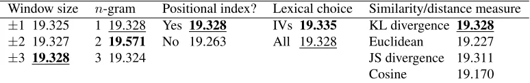
To better understand the sensitivity of the method to each parameter, we perform a post-hoc parame-ter analysis relative to a default setting (as under-lined in Table 2), altering one parameter at a time. The results in Table 2 show that bigrams outper-form other n-gram orders by a large margin (note that the evaluation is based on a log scale), and information-theoretic measures are superior to the geometric measures. Furthermore, it also indicates using the positional indexing better captures context. However, there is little to distinguish context mod-elling with just IV words or all tokens. Similarly, the context window size has relatively little impact on the overall performance, supporting our earlier observation from Table 1.
5 Pair Re-ranking by String Similarity
Once the contextually-similar (OOV,IV) pairs are generated using the selected parameters in Section 4, we further re-rank this set of pairs in an at-tempt to boost morphophonemically-similar pairs like (bananaz,bananas), and penalise noisy pairs like(paninis,beans).
Instead of using the small 10 million tweet pus, from this step onwards, we use a larger cor-pus of 80 million English tweets (collected over the same period as the development corpus) to develop a larger-scale normalisation dictionary. This is be-cause once pairs are generated, re-ranking based on string comparison is much faster. We only include in the dictionary OOV words with a token frequency >15to include more OOV types than in Section 4, and again apply a minimum length cutoff of 4 char-acters.
normal-Rank Window size n-gram Positional index? Lex. choice Sim/distance measure log(CG)
1 ±3 2 Yes All KL divergence 19.571
2 ±3 2 No All KL divergence 19.562
3 ±2 2 Yes All KL divergence 19.562
4 ±3 2 Yes IVs KL divergence 19.561
[image:6.612.113.500.167.228.2]5 ±2 2 Yes IVs JS divergence 19.554
Table 1: The five best parameter combinations in the exhaustive search of parameter combinations
Window size n-gram Positional index? Lexical choice Similarity/distance measure
±1 19.325 1 19.328 Yes 19.328 IVs 19.335 KL divergence 19.328
±2 19.327 2 19.571 No 19.263 All 19.328 Euclidean 19.227
±3 19.328 3 19.324 JS divergence 19.311 Cosine 19.170
Table 2: Parameter sensitivity analysis measured aslog(CG)for correctly-generated pairs. We tune one parameter at a time, using the default (underlined) setting for other parameters; the non-exhaustive best-performing setting in each case is indicated inbold.
isations for lexical variants, e.g. (bcuz,cause)), we modify our evaluation metric from Section 4 to evaluate the rankingat different points, using Dis-counted Cumulative Gain (DCG@N: Jarvelin and Kekalainen (2002)):
DCG@N =rel1+ N
X
i=2
reli
log2(i)
where reli again represents the frequency of the
OOV, but it can be gain (a positive number) or loss (a negative number), depending on whether the ith pair is correct or incorrect. Because we also expect correct pairs to be ranked higher than incorrect pairs, DCG@N takes both factors into account.
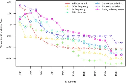
Given the generated pairs and the evaluation met-ric, we first consider three baselines: no re-ranking (i.e., the final ranking is that of the contextual simi-larity scores), and re-rankings of the pairs based on the frequencies of the OOVs in the Twitter corpus, and the IV unigram frequencies in the Google Web 1T corpus (Brants and Franz, 2006) to get less-noisy frequency estimates. We also compared a variety of re-rankings based on a number of string similarity measures that have been previously considered in normalisation work (reviewed in Section 2). We ex-periment with standard edit distance (Levenshtein, 1966), edit distance over double metaphone codes (phonetic edit distance: (Philips, 2000)), longest common subsequence ratio over the consonant edit distance of the paired words (hereafter, denoted as
consonant edit distance: (Contractor et al., 2010)), and a string subsequence kernel (Lodhi et al., 2002). In Figure 1, we present the DCG@N results for each of our ranking methods at different rank cut-offs. Ranking by OOV frequency is motivated by the assumption that lexical variants are frequently used by social media users. This is confirmed by our findings that lexical pairs like (goin,going)
and (nite,night) are at the top of the ranking. However, many proper nouns and named entities are also used frequently and ranked at the top, mixed with lexical variants like(Facebook,speech)
and (Youtube,web). In ranking by IV word fre-quency, we assume the lexical variants are usually derived from frequently-used IV equivalents, e.g.
(abou,about). However, many less-frequent lexical variant types have high-frequency (IV) normalisa-tions. For instance, the highest-frequency IV word
thehas more than 40 OOV lexical variants, such as
ttheandthhe. These less-frequent types occupy the top positions, reducing the cumulative gain. Com-pared with these two baselines, ranking by default contextual similarity scores delivers promising re-sults. It successfully ranks many more intuitive nor-malisation pairs at the top, such as (2day,today)
and(wknd,weekend), but also ranks some incorrect pairs highly, such as(needa,gotta).
dis-tance ranking is fairly accurate for lexical vari-ants with low edit distance to their standard forms, but fails to identify heavily-altered variants like
(tmrw,tomorrow). Consonant edit distance is simi-lar to standard edit distance, but places many longer words at the top of the ranking. Edit distance over double metaphone codes (phonetic edit dis-tance) performs particularly well for lexical vari-ants that include character repetitions — commonly used for emphasis on Twitter — because such rep-etitions do not typically alter the phonetic codes. Compared with the other methods, the string subse-quence kernel delivers encouraging results. It mea-sures common character subsequences of length n between (OOV,IV) pairs. Because it is computa-tionally expensive to calculate similarity for larger n, we choose n=2, following Gouws et al. (2011). As N (the lexicon size cut-off) increases, the per-formance drops more slowly than the other meth-ods. Although this method fails to rank heavily-altered variants such as(4get,forget)highly, it typi-cally works well for longer words. Given that we fo-cus on longer OOVs (specifically those longer than 4 characters), this ultimately isn’t a great handicap.
6 Evaluation
Given the re-ranked pairs from Section 5, here we apply them to a token-level normalisation task us-ing the normalisation dataset of Han and Baldwin (2011).
6.1 Metrics
We evaluate using the standard evaluation metrics of precision (P), recall (R) and F-score (F) as detailed below. We also consider the false alarm rate (FA) and word error rate (WER), also as shown below. FA measures the negative effects of applying nor-malisation; a good approach to normalisation should not (incorrectly) normalise tokens that are already in their standard form and do not require normalisa-tion.6WER, like F-score, shows the overall benefits of normalisation, but unlike F-score, measures how many token-level edits are required for the output to be the same as the ground truth data. In general, dic-tionaries with a high F-score/low WER and low FA
6FA + P≤1 because some lexical variants might be incor-rectly normalised.
are preferable.
P = # correctly normalised tokens
# normalised tokens
R = # correctly normalised tokens
# tokens requiring normalisation
F = 2P R
P+R
FA = # incorrectly normalised tokens
# normalised tokens
WER = # token edits needed after normalisation
# all tokens
6.2 Results
We select the three best re-ranking methods, and best cut-off N for each method, based on the highest DCG@N value for a given method over the development data, as presented in Figure 1. Namely, they are string subsequence kernel (S-dict, N=40,000), double metaphone edit distance (DM-dict, N=10,000) and default contextual similarity without re-ranking (C-dict,N=10,000).7
We evaluate each of the learned dictionaries in Ta-ble 3. We also compare each dictionary with the performance of the manually-constructed Internet slang dictionary (HB-dict) used by Han and Bald-win (2011), the small automatically-derived dictio-nary of Gouws et al. (2011) (GHM-dict), and com-binations of the different dictionaries. In addition, the contribution of these dictionaries in hybrid nor-malisation approaches is also presented, in which we first normalise OOVs using a given dictionary (com-bined or otherwise), and then apply the normalisa-tion method of Gouws et al. (2011) based on con-sonant edit distance (GHM-norm), or the approach of Han and Baldwin (2011) based on the summation of many unsupervised approaches (HB-norm), to the remaining OOVs. Results are shown in Table 3, and discussed below.
6.2.1 Individual Dictionaries
Overall, the individual dictionaries derived by the re-ranking methods (DM-dict, S-dict) perform
N cut−offs
Discounted Cum
ulativ
e Gain
10K 30K 50K 70K 90K
110K 130K 150K 170K 190K
−60K −40K −20K 0 20K 40K
Without rerank OOV frequency IV frequency Edit distance
[image:8.612.96.518.58.339.2]Consonant edit dist. Phonetic edit dist. String subseq. kernel
Figure 1: Re-ranking based on different string similarity methods.
ter than that based on contextual similarity (C-dict) in terms of precision and false alarm rate, indicating the importance of re-ranking. Even though C-dict delivers higher recall — indicating that many lexi-cal variants are correctly normalised — this is offset by its high false alarm rate, which is particularly un-desirable in normalisation. Because S-dict has better performance than DM-dict in terms of both F-score and WER, and a much lower false alarm rate than C-dict, subsequent results are presented using S-dict only.
Both HB-dict and GHM-dict achieve better than 90% precision with moderate recall. Compared to these methods, S-dict is not competitive in terms of either precision or recall. This result seems rather discouraging. However, considering that S-dict is an automatically-constructed dictionary targeting lexi-cal variants of varying frequency, it is not surprising that the precision is worse than that of HB-dict — which is manually-constructed — and GHM-dict — which includes entries only for more-frequent OOVs for which distributional similarity is more accurate. Additionally, the recall of S-dict is hampered by the
restriction on lexical variant token length of 4 char-acters.
6.2.2 Combined Dictionaries
Next we look to combining HB-dict, GHM-dict and S-dict. In combining the dictionaries, a given OOV word can be listed with different standard forms in different dictionaries. In such cases we use the following preferences for dictionaries — moti-vated by our confidence in the normalisation pairs of the dictionaries — to resolve conflicts: HB-dict >GHM-dict>S-dict.
sub-Method Precision Recall F-Score False Alarm Word Error Rate
C-dict 0.474 0.218 0.299 0.298 0.103
DM-dict 0.727 0.106 0.185 0.145 0.102
S-dict 0.700 0.179 0.285 0.162 0.097
HB-dict 0.915 0.435 0.590 0.048 0.066
GHM-dict 0.982 0.319 0.482 0.000 0.076
HB-dict+S-dict 0.840 0.601 0.701 0.090 0.052
GHM-dict+S-dict 0.863 0.498 0.632 0.072 0.061
HB-dict+GHM-dict 0.920 0.465 0.618 0.045 0.063
HB-dict+GHM-dict+S-dict 0.847 0.630 0.723 0.086 0.049
GHM-dict+GHM-norm 0.338 0.578 0.427 0.458 0.135
HB-dict+GHM-dict+S-dict+GHM-norm 0.406 0.715 0.518 0.468 0.124
HB-dict+HB-norm 0.515 0.771 0.618 0.332 0.081
[image:9.612.320.535.319.418.2]HB-dict+GHM-dict+S-dict+HB-norm 0.527 0.789 0.632 0.332 0.079
Table 3: Normalisation results using our derived dictionaries (contextual similarity (C-dict); double metaphone ren-dering (DM-dict); string subsequence kernel scores (S-dict)), the dictionary of Gouws et al. (2011) (GHM-dict), the Internet slang dictionary (HB-dict) from Han and Baldwin (2011), and combinations of these dictionaries. In addition, we combine the dictionaries with the normalisation method of Gouws et al. (2011) (GHM-norm) and the combined unsupervised approach of Han and Baldwin (2011) (HB-norm).
stantially over HB-dict and GHM-dict, respectively, indicating that S-dict contains markedly different entries to both HB-dict and GHM-dict. The best F-score and WER are obtained using the combination of all three dictionaries, HB-dict+GHM-dict+S-dict. Furthermore, the difference between the results us-ing dict+S-dict and HB-dict+GHM-dict is statistically significant (p < 0.01), based on the computationally-intensive Monte Carlo method of Yeh (2000), demonstrating the contribution of S-dict.
6.2.3 Hybrid Approaches
The methods of Gouws et al. (2011) (i.e. GHM-dict+GHM-norm) and Han and Baldwin (2011) (i.e. HB-dict+HB-norm) have lower preci-sion and higher false alarm rates than the dictionary-based approaches; this is largely caused by lex-ical variant detection errors.8 Using all dic-tionaries in combination with these methods — dict+GHM-dict+S-dict+GHM-norm and HB-dict+GHM-dict+S-dict+HB-norm — gives some improvements, but the false alarm rates remain high. Despite the limitations of a pure dictionary-based approach to normalisation — discussed in Section 3.1 — the current best practical approach to
normal-8
Here we report results that do not assume perfect detection of lexical variants, unlike the original published results in each case.
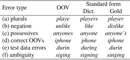
Error type OOV Standard form Dict. Gold (a) plurals playe players player (b) negation unlike like dislike (c) possessives anyones anyone anyone’s (d) correct OOVs iphone phone iphone (e) test data errors durin during durin (f) ambiguity siging signing singing
Table 4: Error types in the combined dictionary (HB-dict+GHM-dict+S-dict)
isation is to use a lexicon, combining hand-built and automatically-learned normalisation dictionaries.
6.3 Discussion and Error Analysis
remain-Length cut-off (N) #Variants Precision Recall (≥N) Recall (all) False Alarm
≥4 556 0.700 0.381 0.179 0.162
≥5 382 0.814 0.471 0.152 0.122
≥6 254 0.804 0.484 0.104 0.131
≥7 138 0.793 0.471 0.055 0.122
Table 5: S-dict normalisation results broken down according to OOV token length. Recall is presented both over the subset of instances of length≥N in the data (“Recall (≥N)”), and over the entirety of the dataset (“Recall (all)”); “#Variants” is the number of token instances of the indicated length in the test dataset.
ing miscellaneous error isbday“birthday”, which is mis-normalised asday.
To further study the influence of OOV word length relative to the normalisation performance, we conduct a fine-grained analysis of the performance of the derived dictionary (S-dict) in Table 5, bro-ken down across different OOV word lengths. The results generally support our hypothesis that our method works better for longer OOV words. The derived dictionary is much more reliable for longer tokens (length 5, 6, and 7 characters) in terms of pre-cision and false alarm. Although the recall is rela-tively modest, in the future we intend to improve re-call by mining more normalisation pairs from larger collections of microblog data.
7 Conclusions and Future Work
In this paper, we describe a method for automat-ically constructing a normalisation dictionary that supports normalisation of microblog text through di-rect substitution of lexical variants with their stan-dard forms. After investigating the impact of dif-ferent distributional and string similarity methods on the quality of the dictionary, we present ex-perimental results on a standard dataset showing that our proposed methods acquire high quality
(lexical variant,standard form) pairs, with reason-able coverage, and achieve state-of-the-art end-to-end lexical normalisation performance on a real-world token-level task. Furthermore, this dictionary-lookup method combines the detection and normali-sation of lexical variants into a simple, lightweight solution which is suitable for processing of high-volume microblog feeds.
In the future, we intend to improve our dictionary by leveraging the constantly-growing volume of mi-croblog data, and considering alternative ways to combine distributional and string similarity. In
addi-tion to direct evaluaaddi-tion, we also want to explore the benefits of applying normalisation for downstream social media text processing applications, e.g. event detection.
Acknowledgements
We would like to thank the three anonymous re-viewers for their insightful comments, and Stephan Gouws for kindly sharing his data and discussing his work.
NICTA is funded by the Australian government as represented by Department of Broadband, Com-munication and Digital Economy, and the Australian Research Council through the ICT centre of Excel-lence programme.
References
AiTi Aw, Min Zhang, Juan Xiao, and Jian Su. 2006. A phrase-based statistical model for SMS text normal-ization. InProceedings of COLING/ACL 2006, pages 33–40, Sydney, Australia.
Edward Benson, Aria Haghighi, and Regina Barzilay. 2011. Event discovery in social media feeds. In Pro-ceedings of the 49th Annual Meeting of the Associa-tion for ComputaAssocia-tional Linguistics: Human Language Technologies (ACL-HLT 2011), pages 389–398, Port-land, Oregon, USA.
Thorsten Brants and Alex Franz. 2006. Web 1T 5-gram Version 1.
Eric Brill and Robert C. Moore. 2000. An improved error model for noisy channel spelling correction. In Proceedings of the 38th Annual Meeting of the Associ-ation for ComputAssoci-ational Linguistics, pages 286–293, Hong Kong.
Danish Contractor, Tanveer A. Faruquie, and L. Venkata Subramaniam. 2010. Unsupervised cleansing of noisy text. InProceedings of the 23rd International Confer-ence on Computational Linguistics (COLING 2010), pages 189–196, Beijing, China.
Paul Cook and Suzanne Stevenson. 2009. An unsu-pervised model for text message normalization. In CALC ’09: Proceedings of the Workshop on Computa-tional Approaches to Linguistic Creativity, pages 71– 78, Boulder, USA.
Jennifer Foster, Ozlem C¨ ¸ etinoglu, Joachim Wagner, Joseph L. Roux, Stephen Hogan, Joakim Nivre, Deirdre Hogan, and Josef van Genabith. 2011. #hard-toparse: POS Tagging and Parsing the Twitterverse. In Analyzing Microtext: Papers from the 2011 AAAI Workshop, volume WS-11-05 of AAAI Workshops, pages 20–25, San Francisco, CA, USA.
Kevin Gimpel, Nathan Schneider, Brendan O’Connor, Dipanjan Das, Daniel Mills, Jacob Eisenstein, Michael Heilman, Dani Yogatama, Jeffrey Flanigan, and Noah A. Smith. 2011. Part-of-speech tagging for Twitter: Annotation, features, and experiments. In Proceedings of the 49th Annual Meeting of the Asso-ciation for Computational Linguistics: Human Lan-guage Technologies (ACL-HLT 2011), pages 42–47, Portland, Oregon, USA.
Roberto Gonz´alez-Ib´a˜nez, Smaranda Muresan, and Nina Wacholder. 2011. Identifying sarcasm in Twitter: a closer look. In Proceedings of the 49th Annual Meeting of the Association for Computational Lin-guistics: Human Language Technologies (ACL-HLT 2011), pages 581–586, Portland, Oregon, USA. Stephan Gouws, Dirk Hovy, and Donald Metzler. 2011.
Unsupervised mining of lexical variants from noisy text. InProceedings of the First workshop on Unsu-pervised Learning in NLP, pages 82–90, Edinburgh, Scotland, UK.
Bo Han and Timothy Baldwin. 2011. Lexical normal-isation of short text messages: Makn sens a #twitter. InProceedings of the 49th Annual Meeting of the As-sociation for Computational Linguistics: Human Lan-guage Technologies (ACL-HLT 2011), pages 368–378, Portland, Oregon, USA.
K. Jarvelin and J. Kekalainen. 2002. Cumulated gain-based evaluation of IR techniques. ACM Transactions on Information Systems, 20(4).
Long Jiang, Mo Yu, Ming Zhou, Xiaohua Liu, and Tiejun Zhao. 2011. Target-dependent Twitter sentiment clas-sification. InProceedings of the 49th Annual Meeting of the Association for Computational Linguistics: Hu-man Language Technologies (ACL-HLT 2011), pages 151–160, Portland, Oregon, USA.
Joseph Kaufmann and Jugal Kalita. 2010. Syntactic nor-malization of Twitter messages. InInternational
Con-ference on Natural Language Processing, Kharagpur, India.
S. Kullback and R. A. Leibler. 1951. On information and sufficiency.Annals of Mathematical Statistics, 22:49– 86.
John D. Lafferty, Andrew McCallum, and Fernando C. N. Pereira. 2001. Conditional random fields: Probabilis-tic models for segmenting and labeling sequence data. InProceedings of the Eighteenth International Confer-ence on Machine Learning, pages 282–289, San Fran-cisco, CA, USA.
Vladimir I. Levenshtein. 1966. Binary codes capable of correcting deletions, insertions, and reversals. Soviet Physics Doklady, 10:707–710.
Mu Li, Yang Zhang, Muhua Zhu, and Ming Zhou. 2006. Exploring distributional similarity based models for query spelling correction. In Proceedings of COL-ING/ACL 2006, pages 1025–1032, Sydney, Australia. Jianhua Lin. 1991. Divergence measures based on the
shannon entropy. IEEE Transactions on Information Theory, 37(1):145–151.
Dekang Lin. 1998. Automatic retrieval and cluster-ing of similar words. InProceedings of the 36th An-nual Meeting of the ACL and 17th International Con-ference on Computational Linguistics (COLING/ACL-98), pages 768–774, Montreal, Quebec, Canada. Fei Liu, Fuliang Weng, Bingqing Wang, and Yang Liu.
2011a. Insertion, deletion, or substitution? normal-izing text messages without pre-categorization nor su-pervision. InProceedings of the 49th Annual Meeting of the Association for Computational Linguistics: Hu-man Language Technologies (ACL-HLT 2011), pages 71–76, Portland, Oregon, USA.
Xiaohua Liu, Shaodian Zhang, Furu Wei, and Ming Zhou. 2011b. Recognizing named entities in tweets. InProceedings of the 49th Annual Meeting of the As-sociation for Computational Linguistics: Human Lan-guage Technologies (ACL-HLT 2011), pages 359–367, Portland, Oregon, USA.
Fei Liu, Fuliang Weng, and Xiao Jiang. 2012. A broad-coverage normalization system for social media lan-guage. In Proceedings of the 50th Annual Meeting of the Association for Computational Linguistics (ACL 2012), Jeju, Republic of Korea.
Huma Lodhi, Craig Saunders, John Shawe-Taylor, Nello Cristianini, and Chris Watkins. 2002. Text classifica-tion using string kernels.J. Mach. Learn. Res., 2:419– 444.
Brendan O’Connor, Michel Krieger, and David Ahn. 2010. TweetMotif: Exploratory search and topic sum-marization for Twitter. InProceedings of the 4th In-ternational Conference on Weblogs and Social Media (ICWSM 2010), pages 384–385, Washington, USA. Lawrence Philips. 2000. The double metaphone search
algorithm. C/C++ Users Journal, 18:38–43.
Lawrence R. Rabiner. 1989. A tutorial on hidden Markov models and selected applications in speech recognition. Proceedings of the IEEE, 77(2):257–286. Alan Ritter, Colin Cherry, and Bill Dolan. 2010. Un-supervised modeling of Twitter conversations. In Proceedings of Human Language Technologies: The 11th Annual Conference of the North American Chap-ter of the Association for Computational Linguistics (NAACL-HLT 2010), pages 172–180, Los Angeles, USA.
Alan Ritter, Sam Clark, Mausam, and Oren Etzioni. 2011. Named entity recognition in tweets: An ex-perimental study. InProceedings of the 2011 Confer-ence on Empirical Methods in Natural Language Pro-cessing (EMNLP 2011), pages 1524–1534, Edinburgh, Scotland, UK.
Takeshi Sakaki, Makoto Okazaki, and Yutaka Matsuo. 2010. Earthquake shakes Twitter users: real-time event detection by social sensors. InProceedings of the 19th International Conference on the World Wide Web (WWW 2010), pages 851–860, Raleigh, North Carolina, USA.
Crispin Thurlow. 2003. Generation txt? The sociolin-guistics of young people’s text-messaging. Discourse Analysis Online, 1(1).
Kristina Toutanova and Robert C. Moore. 2002. Pro-nunciation modeling for improved spelling correction. In Proceedings of the 40th Annual Meeting of the ACL and 3rd Annual Meeting of the NAACL (ACL-02), pages 144–151, Philadelphia, USA.
Official Blog Twitter. 2011. 200 million tweets per day. Retrived at August 17th, 2011.
Jianshu Weng and Bu-Sung Lee. 2011. Event detection in Twitter. In Proceedings of the 5th International Conference on Weblogs and Social Media (ICWSM 2011), Barcelona, Spain.
Zhenzhen Xue, Dawei Yin, and Brian D. Davison. 2011. Normalizing microtext. InProceedings of the AAAI-11 Workshop on Analyzing Microtext, pages 74–79, San Francisco, USA.