On An Interpretation Of Spectral Clustering
Via Heat Equation And Finite Elements Theory
Sandrine Mouysset, Joseph Noailles and Daniel Ruiz
∗Abstract— Spectral clustering methods use eigen-vectors of a matrix, called Gaussian affinity matrix, in order to define a low-dimensional space in which data points can be clustered. This matrix is widely used and depends on a free parameter σ. It is usually in-terpreted as some discretization of the Heat Equation Green kernel. Combining tools from Partial Differen-tial Equations and Finite Elements theory, we propose an interpretation of this spectral method which offers an alternative point of view on how spectral clustering works. This approach develops some particular geo-metrical properties inherent to eigenfunctions of some specific partial differential equation problem. We an-alyze experimentally how this geometrical property is recovered in the eigenvectors of the affinity matrix and we also study the influence of the parameter σ.
Keywords: Clustering, Machine Learning, Spatial Data Mining
1
Introduction
Clustering aims to partition a data set by grouping sim-ilar elements into subsets. Two general main issues con-cern, on the one hand, the choice of a similarity criterion and, on the other hand, how to separate clusters the one from the other. Spectral methods, and in particular the spectral clustering algorithm introduced by Ng-Jordan-Weiss (NJW) [8], are useful when considering non-convex shaped subsets of points. Spectral clustering (SC) con-sists in defining a low-dimensional data space by select-ing particular eigenvectors of a matrix called normalized affinity matrix in which data points are clustered. In this clustering method, two main problems arise : first, what sense can we give to the notion of cluster when con-sidering finite discrete data sets and then, how can we link these clusters to some spectral elements (eigenval-ues/eigenvectors extracted in SC).
Spectral Clustering can be analyzed using graph theory and some normalized cut criterion leading to the solution of some trace-maximum problems (see, for instance, [8], [9]). As the aim is to group data points in some sense of closeness, Spectral Clustering can also be interpreted by exploiting the neighbourhood property in the discretiza-tion of the Laplace-Beltrami operator and heat kernel on
∗IRIT-ENSEEIHT, 2 rue Charles Camichel,
University of Toulouse, France, 31017 BP 122
{sandrine.mouysset,joseph.noailles,daniel.ruiz}@enseeiht.fr
manifolds [2] : in the algorithm, neighbourhood property is represented by the step of adjacency graph. Moreover, consistency of the method was investigated by consider-ing the asymptotic behaviour of clusterconsider-ing when samples become very large [11, 10]. Some properties under stan-dard assumptions for the normalized Laplacian matrices were proved, including convergence of the first eigenvec-tors to eigenfunctions of some limit operator [11, 7]. To the best of our knowledge, the main results establish this relation for huge numbers of points. However, from a nu-merical point of view, SC still works for smaller data sets. So, in this paper, we try to give explanations that may address a given data sample.
A second problem appears when considering the most widely used affinity matrix in spectral clustering tech-niques, as in the NJW-algorithm. It is based on the Gaussian measure between points which depends on a free scale parameterσwhich has to be properly defined. Many investigations on this parameter were led and sev-eral definitions were suggested either heuristically [12, 3], or with physical considerations [6], or from geometrical point of views [5]. The difficulty to fix this choice seems to be tightly connected to the lack of some clustering prop-erty explaining how the grouping in this low-dimensional space defines correctly the partitioning in the original data. We will show how this free parameter affects clus-tering results.
In this paper, as spectral elements used in SC do not give explicitly this topological criteria for a discrete data set, we are drawing back to some continuous formula-tion wherein clusters will appear as disjoint subsets. So eigenvectors of the affinity matrixAwill be interpreted as eigenfunctions of some operator. This drawback is per-formed (section 3) using Finite Elements (FE). Indeed, with FE whose nodes correspond to data points, repre-sentation of anyL2-function is given by its nodal value. So we expect to interpret bothAand its eigenvectors as a representation of respectively aL2operator andL2 func-tions on some bounded regular Ω.
Now, the commonly used operator whose Finite Elements representation matches withA is the kernel of the Heat equation on unbounded space (noted KH). As its
spec-trum is essential, we cannot interpret eigenvectors of A as a representation of eigenfunctions ofKH. However, on a
bounded domainO,KHis closed toKD, the kernel of the
strictly O (section 2.2). Now, operatorSD (convolution
by KD) has eigenfunctions (vni) in H
1
0(Ω). From this, we show (proposition 1) that operator SH (convolution
by KH) admits these vni as near eigenfunctions plus a
residue (notedη). At last, using Finite Elements approx-imation, we show (proposition 2) that eigenvectors of A are a representation of these eigenfunctions plus a residue (noted ψ).
To summarize, the main result of this paper is that for a fixed data set of points, the eigenvectors of A are the representation of functions which support is included in only one connected component at once. The accuracy of this representation is shown to depend for a fixed den-sity of points, on the affinity parameter t. This result is illustrated with small fixed data points (section 4).
1.1
Spectral clustering Algorithm
Let us first give some notations and recall the NJW algo-rithm for anpoints data set in ap-dimensional euclidean space. Assume that the number of targeted clusters kis known. The algorithm contains few steps which are de-scribed as follows:
Algorithm 1Spectral Clustering Algorithm Input : data set, number of clustersk
1. Form the affinity matrixA∈Rn×n defined by:
Aij =
{
exp
(
−∥xi−xj∥2
2σ2 )
ifi̸=j,
0otherwise,
(1)
2. Construct the normalized matrix:
L=D−1/2AD−1/2withDi,i=
∑n
j=1Aij,
3. Assemble the matrix X = [X1X2..Xk] ∈ Rn×k by
stacking those eigenvectors associated with the k
largest eigenvalues ofL,
4. Form the matrix Y by normalizing each row in the
n×k matrix X,
5. Treat each row of Y as a point in Rk, and group
them inkclusters via theK-means method,
6. Assign the original pointxi to clusterj when rowi
of matrix Y belongs to clusterj.
In this paper, we won’t take into account the normal-ization of the affinity matrix described in step 2. But we focus on the two main steps of this algorithm: as-sembling the Gaussian affinity matrix and extracting its eigenvectors to create the low-dimensional space.
2
Clustering property of Heat kernel
As recalled in introduction, Spectral Clustering consists in selecting particular eigenvectors of the normalized affinity matrix defined by (1). Gaussian affinity coeffi-cients Aij are usually interpreted as a representation of
the Heat kernel evaluated at data pointsxi andxj.
Let KH(t, x, y) = (4πt)−
p
2 exp
(
−∥x−y∥2
4t
)
be the Heat kernel in R∗+×Rp×Rp. Note that the Gaussian affinity
between two distinct data points xi and xj is defined
byAij = (2πσ2)−
p
2 KH(σ2/2, xi, xj). Now, consider the
initial value problem inL2(Rp), forf ∈L2(Rp):
(PRp)
{
∂tu−∆u= 0 for (x, t)∈Rp×R+\{0},
u(x,0) =f forx∈Rp,
and introduce the solution operator in L2(Rp)of(P
Rp):
(SH(t)f)(x) =
∫
Rp
KH(t, x, y)f(y)dy, x∈Rp. (2)
Now if f(y)≈δxj(y), whereδxj denotes the Dirac
func-tion on xj, one can observe that:
(
SH(
σ2
2 )f
)
(xi)≈KH
(
σ2
2 , xi−xj
)
=(2πσ2)
p
2 (A+I
n)ij.
Thus, the spectral properties of matrix A used in the Spectral clustering algorithm seems to be related to those of operator SH(t). We propose to analyze this in details
in the following.
2.1
Heat equation with Dirichlet boundary
conditions
To simplify, we shall fix in the following the number of clusterskto 2, but the discussion can be extended to any arbitrary numberk. Consider then a bounded open setΩ
inRpmade up of two disjoint connected open subsetsΩ
1 andΩ2. Assume that the boundary∂Ω =∂Ω1∪∂Ω2with
∂Ω1∩∂Ω2=∅is regular enough so that the trace operator is well-posed on∂Ω and the spectrum decomposition of Laplacian operator is well-defined. For instance, ∂Ω is
C1 on both∂Ω1 and∂Ω2. According to [4], determining the eigenvalues(λn(Ω))n>0and associated eigenfunctions
(vn)n>0 of the Dirichlet Laplacian onΩ:
(PΩL)
{
∆vn=λvn inΩ,
vn = 0on∂Ω,
is equivalent to define a function of the eigenvalues
(λn1(Ω1))n1>0 and (λn2(Ω2))n2>0 and of the
eigenfunc-tions of the Dirichlet Laplacian on Ω1 and Ω2 respec-tively. In other words, if vn ∈ H01(Ω), then ∆v = λv on Ω if and only if for i ∈ {1,2}, vi = v|Ωi ∈H
1 0(Ωi)
{λn1(Ω1)}n1>0∪ {λn2(Ω2)}n2>0. Additionally, if we
con-sider vni the solution on Ωi of P
L
Ωi, an eigenfunction of
the Laplacian operator ∆ associated to λni, and if we
extend the support ofvni ∈Ωito the whole setΩby
set-tingvni = 0inΩ\Ωi, we also get an eigenfunction of the
Laplacian∆ inH1
0(Ω) associated to the same eigenvalue
λni. Note that sinceΩ1 and Ω2 are disjoint, the
exten-sion by 0 to the whole set Ω of any function inH1 0(Ωi)
is a function in H1
0(Ω). Consequently, the union of the two sets of eigenfunctions {(vni)ni>0, i∈ {1,2}}, is an
Hilbert basis ofH1 0(Ω).
Now let f ∈L2(Ω) and consider the heat problem with Dirichlet conditions on the bounded setΩ = Ω1∪Ω2:
(PΩD)
∂tu−∆u= 0in R+×Ω,
u= 0, onR+×∂Ω, u(t= 0) =f, inΩ.
Denote byKDΩ the Green’s kernel of(PΩD). The solution operator in H2(Ω)∩H1
0(Ω)) associated to this problem is defined, for f ∈L2(Ω), by:
SΩD(t)f(x) =
∫
Ω
KD(t, x, y)f(y)dy, x∈Rp.
Eigenfunctions of SΩ
D(t) and those of the Laplacian
op-erator ∆ are the same. Indeed, if vni is an
eigenfunc-tion of (PL
Ω)associated to an eigenvalueλni thenvni is
also eigenfunction of SD(t) with eigenvalue etλni in the
sense that SΩ
D(t)vni(x) =e
tλniv
ni(x). Thus the
geomet-rical property of the eigenfunction is preserved, i.e the support of eigenfunctions can be defined in only one con-nected componentΩ1or Ω2.
2.2
A clustering property from
eigenfunc-tions of Heat equation with Dirichlet
boundary conditions
We consider now the solution operator SH(t) of (PRp).
As opposed to the previous case, we can not deduce sim-ilar properties as with the operator solution of (PΩD) be-cause the spectrum of SH(t) is essential and
eigenfunc-tions are not localized in Rp without boundary condi-tions. However, we are going to compare, for fixed values oft,SH(t)andSDΩ(t)and derive some asymptotic
prop-erties onSH(t)that approximate the previously analyzed
properties of SΩ
D(t).
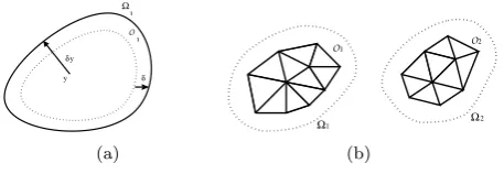
Forε >0, let introduce an open subsetOwhich approx-imates from the interior the open set Ω, in the sense that O ⊂O ⊂¯ Ωand Volume(Ω\O)≤ε. Noteδ(y)the distance of a pointy∈ Oto∂Ω, the boundary ofΩ, and
δ= infy∈Oδ(y)the distance from O toΩ (see fig1). At
last, Ois supposed to be chosen such thatδ >0.
As recalled in [1], fort >0,xandy inΩ,KH(t, x, y)is a
distribution that corresponds to the elementary solutions
O
1 1
δ y
y δ
Ω
(a)
O
2 1
Ω Ω
1
2
O
(b)
Figure 1: (a) Approximation ofΩ1with an open setO1,
(b) Mesh representation : xi∈
◦
Ω, ∀i∈ {1, ..n}
of the heat equation (PRp)|Ω, KH is strictly positive on
the boundary ∂Ω and, due to the maximum principle,
KD is bounded above byKH,∀(t, x, y)∈R+×Ω×Ω:
0< KD(t, x, y)< KH(t, x, y). (3)
Furthermore, both Green’s kernelsKH andKDΩi
approx-imate each other on each open set Oi, i ∈ {1,2} and
an estimation about their difference can be given by, ∀(x, y)∈ Oi× Oi, ∀i∈ {1,2}:
0< KH(t, x, y)−KDΩi(t, x, y)≤
1 (4πt)p2
e−δ(4yt)2. (4)
Now, for any f ∈ L2(Θ), let us come back to the heat solutionSH(t)f and restrict its support to the open set
Oi, for i ∈ {1,2}. For any open set Θ, the resulting
restricted operatorSH to Θ, forf ∈L2(Θ) is:
SHΘ(t)f(x) =
(∫
Θ
KH(t, x, y)f(y)dy
)
|Θ, x∈Θ.
At last, define alsoTi, fori ∈ {1,2} as the L2-mapping
from L2(O
i) onto L2(O) which extends the support of
any functionu∈L2(Oi)to the whole setΩwith:
∀u∈L2(Oi), Ti(u) =
{
uinOi,
0 inΩ\Oi
(5)
With these notations, we can then state the following proposition:
Proposition 1 Let i ∈ {1,2}, vfni = Ti(vni|Oi) where
vni is the eigenfunction inH
2(Ω
i)∩H01(Ωi)associated to
exp−λnit for operatorSΩi
D. Then, for t >0, we have the
following result:
SHO(t)vfni = exp−
λnitvf
ni+η(t,vfni), (6)
with∥η(t,vfni)∥L2(O)→0 whent→0, δ→0.
Proof sketch. By triangular inequality, ∥η(t,vfni)∥L2(O) = SOH(t)vfni−exp−
λnitvf
niL2(O) is
bounded above by three terms:
[image:3.595.314.543.74.153.2]. . .SΩi
D(t)Ti(vni|Oi−vni)
+SΩi
D(t)vni−e
−λnitvf ni
L2(O).
On the right side, Ti(vni|Oi−vni) has its support
in-cluded inΩi\OiandsuppΩi\Oitends to∅whenδ→0.
Moreover, operatorSΩi
D(t)tends to identity when t→0.
So both two last terms in the right side of this inequality vanish when(t, δ)→0.
For vni|Oi ∈ L
2(O
i), ∥ς(t, vni|Oi)∥L2(O) = ∥SHO(t)vfni −
SΩi
D(t)vfni∥L2(O)can be bounded above by means of both
equations (3) and (4), fort >0and for alli∈ {1,2}, by :
(4πt)−2p∥vn
i|Oi∥
2
L2(Oi) (
e−δ
2
2tV ol(Oi) +e−
γ2
4tV ol(O)
)
,
withγ= inf
x∈Oj,y∈Oi
∥x−y∥ ≥2δ.
Proposition 1 means that the operatorSHO(t)has ’almost eigenfunctions’ which are exactly those of the Dirichlet problem (PΩD)restricted to Oi ⊂ Ωi. Moreover, it
pre-cises this closeness behaviour with its dependance on t. At last, these eigenfunctions are supported into a sin-gle connected component which means that they can be used to characterize if a point belongs to a given Ωi or
not. Finally, if we consider the behaviour of the function
s7→(4πs)−p2e−
δ(y)2
4s involved in (4), we may assume that
parameter t should be smaller than δ(y)2 for all y ∈ O, and should tend to 0 within a fraction of the distanceδ2 to preserve the asymptotical result of propostion 1.
3
Interpretation of the Spectral
Cluster-ing algorithm with Finite Elements
Introduce Lagrange finite elements so that nodes are the set of NJW algorithm data pointsΣincluded inO ⊂¯ Rp.
Letτhbe a triangulation onO¯ such that : h= max K∈τh
hK,
hK being a characteristic length of triangleK. Meshing
of each part ofOis represented on figure 1 (b). Thus, con-sider a finite decomposition of the domain : O¯ =∪K∈τhK
in which(K, PK,ΣK)satisfies Lagrange finite element
as-sumptions for allK∈τh: Kis a compact, non empty set
of τh such that supp(K)⊂ O, PK is a finite dimension
vector space generated by shape functions(ϕi)isuch that
PK⊂H1(K)andΣ =∪K∈τhΣK.
Let define the finite dimension approximation space:
Vh={w∈ C0( ¯O);∀K∈τh, w|K ∈PK}.
For all i, 1≤i≤n, let the sequence of shape functions ofVh noted(ϕi)i:O →Rwhereϕi=ϕ|K ∈PK satisfied
to: ϕi(xj) =δij, ∀ xj ∈Σ, δij being the Dirac function
of(i, j).
This finite space Vh is generated by the sequence (ϕi)i
with Vh = V ect < (ϕi)i >⊂ L2(O,R). Let Πh the
linear interpolation from L2(O,R) in Vh with the usual
scalar product (·|·)L2. According to this notations, the
Πh-mapping of kernel y 7→ KH(t, x−y) is defined for
t >0 by, ∀y∈ O, ∀1≤j≤n:
Πh(KH(t, x−y)) =
1
(4πt)p2
n
∑
i=1
exp
(
−∥x−xi∥2
t
)
ϕi(y).
Thus, for t >0, the Πh-mapped operatorSOH applied to
eachϕj is,∀1≤j≤n:
Πh(SHO(t)ϕj)(x) =
1
(4πt)p2
n
∑
k=1
( b
AM
)
kj
ϕk(x) +O(h, x),
(7) whereM stands for the mass matrix defined by : Mij =
(ϕi|ϕj)L2 andAb=A+In whereAis the affinity matrix.
So, with the same assumptions as in section 2.2, equation (1) can be formulated via the linear interpolationΠh:
Proposition 2 Let vni be an eigenfunction of S
Ωi
D(t)in
H2(Ω) ∩H1
0(Ω) associated to the eigenvalue exp−λnit
such that SΩi
D(t)vni = exp−
λnitv
ni. Let i ∈ {1,2},
f
vni = Ti(vni|Oi). Then, for Wni = Πhvfni ∈ Vh and
t >0, :
ΠhSOH(t)Wni= exp
−λnitW
ni+ψ(t, h), (8)
where∥ψ(t, h)∥L2(V
h)→0 when(h, t)→0 andδ→0.
Proof sketch. Apply Πh interpolation to the
equa-tion of proposiequa-tion 1. Using linearity and continuity of
Πh and Cauchy-Schwarz inequality, an upper bound of
∥ΠhSHO(t)(Πhvfni−vfni)∥2could be given, for a given
con-stantCΠh>0, by :
CΠh(4πt)
−p
4∥vn
i|Oi∥L2(Oi)V ol(O) 3 2
(
e−δ
2
2t +e−
γ2
4t
)1
2
.
In this approach, we have to estimate the neighbourhood distance δ between Ωi and Oi for i ∈ {1,2}. But this
result totally relies on both the discretization stephand the Gaussian parametert. So we investigate their role in the following numerical experiments.
4
Numerical experiments
Let consider two test cases : one in which clusters can be separated by hyperplanes (see fig 2(a)) and another one in which clusters are embedded (see fig 3(a)). We analyze the influence of parameter t on the difference between discretized eigenfunctions of SDO(t) and eigen-vectors of matrixAMˆ . In figure 2 (b)-(c)-(d) and figure 3 (b)-(c)-(d), we plot the discretized eigenfunction asso-ciated to the first eigenvalue of each connected compo-nent. We also indicate in figure 2 (e)-(f)-(g) the product of these discretized eigenfunctions Wni, fori∈ {1,2,3},
operatorAMˆ orA. Still, to get better insight about this geometrical invariance property, we finally compare the projection coefficients between these discretized eigen-functions Wni with the eigenvectors of AMˆ and A that
maximizes these projection coefficient. In other words, let Wni = Πhvfni ∈ Vh and Xl the eigenvector of AMˆ
such that l = argmaxj(Wni|Xj), the projection
coeffi-cient correponds then toω = |(Wni|Xl)|
∥Wni∥2∥Xl∥2. Since matrix
ˆ
AM depends on the parameter t, we indicate in figure (k) how this coefficient ω evolves with varying values of
t. In figure (l), we also indicate the difference of the norms α=∥Xl−Wni∥2. We do the same in figure (m)
and (n) with respect to eigenvectors of the affinity matrix
A instead of AMˆ and noted respectively τ and β. The projection coefficient ω, which gets close to 1 for some optimal value of t, highlights the fact discretized eigen-functions of Laplacian operator with Dirichlet boundary conditions on some wider subsetΩithat includes the
con-nected componentOi are indeed close to eigenvectors of
the discretized heat operator without boundary condi-tions but with a parametert that needs to be chosen in a given appropriate window.
The vertical dash-dot line in figure (k)-(l)-(m)-(n) in-dicates the value of the parameter t based on the geo-metrical point of view proposed in [5]: th = Dmax
2np1
with
Dmax = max1≤i,j≤n∥xi−xj∥2. At a first glance, it is
close to an optimum in all these figures. This critical value th, seems to give a good estimate of the length
δ between clusters. This critical value th relies on the
assumption that the p-dimensional data set is isotropic enough in the sense that no directions are privileged with very different magnitudes in the distances between points along these directions. It shows the link between eigen-vectors and eigenfunctions with respect to parameter t, and thatthis a good candidate to perform Spectral
Clus-tering.
5
Conclusion
In this paper, we analyze some steps of Spectral Cluster-ing with analogy to eigenvalue problems. From this inter-pretation, a clustering property based on the eigenvectors and an asymptotic condition on the Gaussian parameter have been extracted. This leads to some interpretation on how spectral clustering works and how results could be affected with respect to the affinity parameter and separation between clusters. However we didn’t take into account the normalization step of the spectral clustering algorithm which role is crucial to order the eigenvalues in an appropriate way so that connected components are easy to detect by means of eigenvectors associated to the largest eigenvalues.
−6 −4 −2 0 2 4 6
−6 −4 −2 0 2 4 6 8
(a) Data set
−6 −4−2 0 24 6 −10 −5 0 5 10 −0.05 0 0.05 0.1 0.15 0.2 0 0.02 0.04 0.06 0.08 0.1 0.12 0.14 0.16 (b)
−6 −4 −2 0 2 4
6 −6 −4 −2 0 2 4 6 8 −0.3 −0.2 −0.1 0 0.1 −0.25 −0.2 −0.15 −0.1 −0.05 0 (c)
−6 −4−20 2 4 6 −10 −5 0 5 10 −0.25 −0.2 −0.15 −0.1 −0.05 0 0.05 0.1 −0.2 −0.15 −0.1 −0.05 0 (d)
−6−4−20 246 −10 −5 0 5 100 0.01 0.02 0.03 0.04 0.05 0.06 0.07 0.08 0.09 0.1 0.01 0.02 0.03 0.04 0.05 0.06 0.07 0.08 (e)
−6 −4 −2 0 2 4 6 −6 −4 −2 0 2 4 6 8 −0.1 −0.05 0 −0.08 −0.07 −0.06 −0.05 −0.04 −0.03 −0.02 −0.01 (f)
−6 −4−20 2 4 6 −10 −5 0 5 10 −0.08 −0.07 −0.06 −0.05 −0.04 −0.03 −0.02 −0.01 0 −0.07 −0.06 −0.05 −0.04 −0.03 −0.02 −0.01 (g) −6−4 −202
4 6 −10 −5 0 5 100 0.05 0.1 0.15 0.2 0.25 0.3 0.35 0.4 0.05 0.1 0.15 0.2 0.25 0.3 0.35 (h)
−6 −4 −2 0 2 4 6 −6 −4 −2 0 2 4 6 8 −0.4 −0.3 −0.2 −0.1 0 −0.35 −0.3 −0.25 −0.2 −0.15 −0.1 −0.05 (i)
−6−4−20 24 6 −10 −5 0 5 10 −0.4 −0.35 −0.3 −0.25 −0.2 −0.15 −0.1 −0.05 0 −0.35 −0.3 −0.25 −0.2 −0.15 −0.1 −0.05 (j)
0 0.1 0.2 0.3 0.4 0.5 0.6 0.7 0.8 0.9 0 0.1 0.2 0.3 0.4 0.5 0.6 0.7 0.8 0.9 1 t ω Wn 1 Wn 2 Wn 3 (k)
0 0.1 0.2 0.3 0.4 0.5 0.6 0.7 0.8 0.9 0 0.2 0.4 0.6 0.8 1 t α Wn 1 Wn 2 Wn 3 (l)
0 0.1 0.2 0.3 0.4 0.5 0.6 0.7 0.8 0.9 0 0.1 0.2 0.3 0.4 0.5 0.6 0.7 0.8 0.9 1 t τ Wn 1 Wn 2 Wn 3 (m)
0 0.1 0.2 0.3 0.4 0.5 0.6 0.7 0.8 0.9 0.4 0.5 0.6 0.7 0.8 0.9 1 t β Wn 1 Wn 2 Wn 3 (n)
Figure 2: Example 1: (a) Data set with n= 302points, (b), (c), (d) Discretized eigenfunctionWni, i∈ {1,2,3},
(e)-(f)-(g) Product AM Wˆ ni, (h)-(i)-(j) Product AWni,
(k)-(l) Correlation ω and Euclidean norm difference α
between Wni, i ∈ {1,2,3} and eigenvectors Xl of AMˆ
functions oft, (m)-(n) Correlationτand Euclidean norm difference β between Wni, i∈ {1,2,3} and eigenvectors
−6 −4 −2 0 2 4 6 8 −6 −4 −2 0 2 4 6 8
(a) Data set
−5 0 5 10 −10 −5 0 5 10 −0.25 −0.2 −0.15 −0.1 −0.05 0 0.05 −0.2 −0.15 −0.1 −0.05 0 (b) −5 0 5 −5 0 5 −0.1 −0.08 −0.06 −0.04 −0.02 0 −0.1 −0.09 −0.08 −0.07 −0.06 −0.05 −0.04 −0.03 −0.02 −0.01 0 (c) −4 −20
246 −5 0 5 −0.5 −0.4 −0.3 −0.2 −0.1 0 −0.5 −0.45 −0.4 −0.35 −0.3 −0.25 −0.2 −0.15 −0.1 −0.05 0 (d)
−6−4−202468 −10 −5 0 5 10 −0.05 −0.04 −0.03 −0.02 −0.01 0 −0.045 −0.04 −0.035 −0.03 −0.025 −0.02 −0.015 −0.01 −0.005 (e) −6 −4 −20 2 4 68 −6 −4 −2 0 2 4 6 8 −0.025 −0.02 −0.015 −0.01 −0.005 0 −0.02 −0.015 −0.01 −0.005 (f) −5 0 5 10 −10 −5 0 5 10 −0.05 −0.04 −0.03 −0.02 −0.01 0 −0.045 −0.04 −0.035 −0.03 −0.025 −0.02 −0.015 −0.01 −0.005 (g)
−4−202 46 −5 0 5 −0.25 −0.2 −0.15 −0.1 −0.05 0 −0.25 −0.2 −0.15 −0.1 −0.05 (h) −5 0 5 10 −6 −4 −2 0 2 4 6 8 −0.025 −0.02 −0.015 −0.01 −0.005 0 −0.02 −0.015 −0.01 −0.005 (i) −5 0 5 10 −10 −5 0 5 10 −0.25 −0.2 −0.15 −0.1 −0.05 0 −0.2 −0.18 −0.16 −0.14 −0.12 −0.1 −0.08 −0.06 −0.04 −0.02 (j)
0 0.1 0.2 0.3 0.4 0.5 0.6 0.7 0.8 0.9 0 0.1 0.2 0.3 0.4 0.5 0.6 0.7 0.8 0.9 1 t ω Wn 1 Wn 2 Wn 3 (k)
0 0.1 0.2 0.3 0.4 0.5 0.6 0.7 0.8 0.9 0 0.2 0.4 0.6 0.8 1 t α Wn 1 Wn 2 Wn 3 (l)
0 0.1 0.2 0.3 0.4 0.5 0.6 0.7 0.8 0.9 0 0.1 0.2 0.3 0.4 0.5 0.6 0.7 0.8 0.9 1 t τ Wn 1 Wn 2 Wn 3 (m)
0 0.1 0.2 0.3 0.4 0.5 0.6 0.7 0.8 0.9 0 0.2 0.4 0.6 0.8 1 1.2 t β Wn 1 Wn 2 Wn 3 (n)
Figure 3: Example 2: (a) Data set with n= 368points, (b), (c), (d) Discretized eigenfunction Wni, i∈ {1,2,3},
(e)-(f)-(g) Product AM Wˆ ni, (h)-(i)-(j) Product AWni,
(k)-(l) Correlation ω and Euclidean norm difference α
between Wni, i ∈ {1,2,3} and eigenvectors Xl of AMˆ
functions oft, (m)-(n) Correlationτand Euclidean norm difference β between Wni, i∈ {1,2,3} and eigenvectors
YlofA functions oft.
References
[1] C. Bardos and O. Lafitte. Une synthese de resultats anciens et recents sur le comportement asymptotique des valeurs propres du Laplacien sur une variete rie-mannienne. CMLA, 1998.
[2] M. Belkin and P. Niyogi. Laplacian eigenmaps and spectral techniques for embedding and clustering.
Advances in Neural Information Processing Systems, 14(3), 2002.
[3] M. Brand and K. Huang. A unifying theorem for spectral embedding and clustering.9th International Conference on Artificial Intelligence and Statistics, 2002.
[4] F. Hirsch and G. Lacombe. Elements of functional analysis. Springer, 1999.
[5] S. Mouysset, J. Noailles, and D. Ruiz. Using a Global Parameter for Gaussian Affinity Matrices in Spec-tral Clustering. InHigh Performance Computing for Computational Science: 8th International Confer-ence, Toulouse, France, June 24-27, 2008. Revised Selected Papers, pages 378–391. Springer, 2009.
[6] B. Nadler and M. Galun. Fundamental limitations of spectral clustering. Advances in Neural Information Processing Systems, 19:1017, 2007.
[7] B. Nadler, S. Lafon, R.R. Coifman, and I.G. Kevrekidis. Diffusion maps, spectral clustering and eigenfunctions of fokker-planck operators. Arxiv preprint math/0506090, 2005.
[8] A. Y. Ng, Michael I. Jordan, and Yair Weiss. On spectral clustering: analysis and an algorithm.
Proc.Adv.Neural Info.Processing Systems, 2002.
[9] Jianbo Shi and Jitendra Malik. Normalized cuts and image segmentation. IEEE Transactions on Pattern Analysis and Machine Intelligence, 22(8):888–905, 2000.
[10] U. Von Luxburg, M. Belkin, and O. Bousquet. Con-sistency of spectral clustering. Annals of Statistics, 36(2):555, 2008.
[11] U. Von Luxburg, O. Bousquet, and M. Belkin. Lim-its of spectral clustering. Advances in neural infor-mation processing systems, 17, 2004.