An Overview of A Family of New Iterative Methods Based on IDR Theorem And Its Estimation

Full text

(1)Proceedings of the International MultiConference of Engineers and Computer Scientists 2009 Vol II IMECS 2009, March 18 - 20, 2009, Hong Kong. An Overview of A Family of New Iterative Methods Based on IDR Theorem And Its Estimation Yusuke Onoue. ∗. Abstract—After birth of IDR(s) method based on IDR Theorem, two variants of MR IDR(s) and Bi IDR(s) methods were proposed one after another. The former method gained stability by adoptation of strategy of minimizing intermediate residual norm with extra computational cost. The latter method became sophiscated and elegant variant with stability by means of adoptation of bi-orthogonalization conditions. In this article, we overview a family of IDR(s) methods, and evaluate performance of these variants through several numerical experiments. Keywords: IDR Theorem, IDR(s) method, MR IDR(s) method, Bi IDR(s) method. 1. Introduction. We consider to solve a unsymmetric linear system of equations, Ax = b,. (1). where A is a given unsymmetric coefficient matrix in RN ×N , and x is a solution vector in RN , and b is a right-hand side vector in RN . Krylov subspace methods are effective for solving linear systems of equations [2]. Krylov subspace is defined as follows: Kn (A; r 0 ) :=. †. Seiji Fujino. span{r 0 , Ar 0 , . . . , An−1 r 0 }.. (2). Norimasa Nakashima. ‡. method is competitive with or superior to most producttype BiCG methods, and outperforms BiCGStab method when s > 1. Furthermore, Minimum Residual IDR(s) (MR IDR(s)) and Bi-orthogonalized IDR(s) (Bi IDR(s)) methods are proposed as variants of IDR(s) method one after another by P. Sonneveld and M. B. van Gijzen[6][7]. In this paper, we overview MR IDR(s) and Bi IDR(s) methods, and determine effectiveness of these two iterative methods through numerical experiments. This paper is organized as follows. In section 2, we note outline and algorithm of IDR(s) method. In section 3, we describe outline and algorithm of MR IDR(s) method. In section 4, we describe outline and algorithm of Bi IDR(s) method. In section 5, we examine effectiveness of MR IDR(s) and Bi IDR(s) methods through numerical experiments. Finally, in section 6, we draw concluding remarks.. 2. IDR(s) method. In this section, characteristics of IDR(s) method can be mentioned as follows[5]: IDR Theorem. Here, r 0 := b − Ax0 is an initial residual vector. The members of Krylov subspace methods, product-type BiConjugate Gradient (BiCG) methods are often used for solving nonsymmetric linear systems of equations. BiCG stabilized (BiCGStab) method [2] is one of versions of product-type Bi-Conjugate Gradient (BiCG) methods.. Let A be any matrix in RN ×N , and v 0 be any vector in RN , and G0 be the complete Krylov space KN (A, v 0 ). Let S denote any space in RN , and define the sequence spaces Gj (j = 1, 2, . . .) as. In 2007, one of Krylov subspace method, IDR(s) method is proposed by P. Sonneveld and M. B. van Gijzen [5]. IDR(s) method is based on the IDR Theorem. IDR(s). Here ωj ’s are non-zero scalars. Then, the next two Theorems hold.. ∗ Graduate. School of Information Science and Electrical Engineering, Kyushu University, Email: [email protected] † Research Institute for Information Technology, Kyushu University, Email: [email protected] ‡ Graduate School and Faculty of Information Science and Electrical Engineering, Kyushu University, Email: [email protected]. ISBN: 978-988-17012-7-5. Gj := (I − ωj A)(Gj−1 ∩ S).. (3). (i) Gj ⊆ Gj−1 for all j > 0, (ii) Gj = {0} for some j ≤ N . Computing the first residual r n+1 in Gj+1. IMECS 2009.

(2) Proceedings of the International MultiConference of Engineers and Computer Scientists 2009 Vol II IMECS 2009, March 18 - 20, 2009, Hong Kong. IDR(s) method is built such that s + 1 residual vectors are forced to be in Gj . The reisdual r n+1 is in Gj+1 if r n+1 = (I − ωj A)v n , v n ∈ Gj ∩ Null(P T ).. (4). 7.. End Do. 8.. Es = (es−1 , . . . , e0 ), Qs = (q s−1 , . . . , q 0 ). 9.. Do n = s, s + 1, . . .. 10.. Solve cn from P T En cn = P T r n. Here, parameter ωj is determined by solving minimization of the residual norm ||r n+1 ||2 .. 11.. v n = r n − En cn. 12.. If mod(n, s + 1) = s then. 13.. Computing a combination of the residual vectors, a vector v n. 14.. tn = Av n (tn , v n ) ω= (tn , tn ) ( |(t ,v )| ρ = ||t ||n∗||n v n ||2 n 2 If ρ < κ then ω =. ) κ ω ρ. en = −En cn − ωtn. Vector v n can be written as a combination of the residual vectors in Gj because v n ∈ Gj ∩ Null(P T ). We define the forward difference residual vector en := r n+1 − r n . If r n−i (i = 0, . . . , s) ∈ Gj then en−i (i = 1, . . . , s) ∈ Gj . Thus, vector v n can be written as. 15.. s ∑. 20.. End If. 21.. r n+1 = r n + en , xn+1 = xn + q n. 22.. if ||r n+1 ||2 /||r 0 ||2 ≤ ϵ then stop. vn = rn −. ci en−i .. (5). i=1. Since v n ∈ Null(P T ), it satisfies P T v n = 0. We can solve the coefficients ci by solving an s × s linear system P T v n = 0. Besides, we can compute the vector v n . Computing the kth residual r n+k in subspace Gj+1. q n = −Qn cn + ωv n. 16. 17.. Else q n = −Qn cn + ωv n. 18.. en = −Aq n. 19.. 23.. En+1 = (en , . . . , en+1−s ), Qn+1 = (q n , . . . , q n+1−s ). 24.. End Do. In steps 4th and 14th, we note the additional computation for ω. The computation improves the accuracy of IDR(s) method.. The kth residual r n+k (2 ≤ k ≤ s + 1) can be computed by consecutive computations as follows:. 3. Computing the kth residual r n+k in subspace Gj+1. In this section, characteristics of MR IDR(s) method can be mentioned as follows[7]:. 1.. Solve ci from P T. s ∑. ci en+k−1−i = P T r n+k−1. i=1. 2.. v n+k−1 = r n+k−1 −. MR IDR(s) method. s ∑. ci en+k−1−i. Computing the kth residual r n+k in subspace Gj+1. i=1. 3.. r n+k = (I − ωj A)v n+k−1. Here, r n+k−1−i ∈ Gj+1 ⊆ Gj when 1 ≤ i < k, and r n+k−1−i ∈ Gj when k ≤ i ≤ s. Therefore, en+k−1−i ∈ Gj and r n+k ∈ Gj+1 . We present the algorithm of IDR(s) method as follows:. The kth residual r n+k (1 ≤ k ≤ s + 1) can be computed by consecutive computations as follows: Computing the kth residual r n+k in subspace Gj+1 1.. Solve ci from P T. s ∑. ci g n+k−1−i = P T r n+k−1. i=1. 2.. v n+k−1 = r n+k−1 −. s ∑. ci g n+k−1−i. i=1. Algorithm 1:. 3.. IDR(s) method. 1.. Let x0 be a random vector, and put r 0 = b − Ax0. 2.. For n = 0, . . . , s − 1 Do. 3.. v n = Ar n (v n , r n ) ω= (v n , v n ) ( |(v ,r )| ρ = ||v ||n∗||nr || n 2 n 2 If ρ < κ then ω =. 4.. Here, the vector g n is defined as ) κ ω ρ. en = −ωv n. 5.. q n = ωr n ,. 6.. r n+1 = r n + en , xn+1 = xn + q n. ISBN: 978-988-17012-7-5. r n+k = (I − ωj A)v n+k−1. g n := (−1) ∗ en = r n − r n+1 .. (6). r n+k−1−i ∈ Gj+1 ⊆ Gj when 1 ≤ i < k, and r n+k−1−i ∈ Gj when k ≤ i ≤ s. Accordingly, g n+k−1−i ∈ Gj and r n+k ∈ Gj+1 .. IMECS 2009.

(3) Proceedings of the International MultiConference of Engineers and Computer Scientists 2009 Vol II IMECS 2009, March 18 - 20, 2009, Hong Kong. Minimization of the intermediate residual norms Let matrix Gn+k = (g n+k−1 , . . . , n + k − s). Having computed k orthogonal columns of Gn+k , the kth intermediate residual r n+k can be minimized over the vectors in Gj+1 by making r n+k orthogonal to the first k columns of Gn+k . We present the algorithm of MR IDR(s) method as follows: Algorithm 2:. MR IDR(s) method. 1.. Let x0 be a random vector, and put r 0 = b − Ax0 ,. 2.. G−1 , U−1 = O ∈ RN ×s , M−1 = I, ω0 = 1. 3.. n = 0, j = 0. 4.. While ||r n ||2 /||r 0 ||2 > ϵ Do. 5.. Do k = 1, . . . , s. 6.. m = P T rn. 7.. Solve c from Mj−1 c = m. 8.. v = r n − Gj−1 c, ū = Uj−1 c + ωj v. 9.. ḡ = Aū. 10.. Do i = 1, . . . , k − 1. 11.. α = (g n−i , ḡ). 12. 13.. ḡ = ḡ − αg n−i , ū = ū − αun−i. 16.. End Do √ α = (ḡ, ḡ) 1 1 g n = ḡ, un = ū α α βn = (r n , g n ). 17.. r n+1 = r n − βn g n , xn+1 = xn + βn un. 14. 15.. 18. 19.. n=n+1 End Do. 20.. Gj = (g n−1 , . . . , g n−s ), Uj = (un−1 , . . . , un−s ). 21.. Mj = P T G j , m = P T r n. 22.. Solve c from Mj c = m. 23.. v = r n − Gj c, t = Av. 24.. ωj+1 =. 25.. xn+1. 26.. r n+1 = r n − Gj c − ωj+1 t. 27.. n = n + 1, j = j + 1. 28.. (t, v) (t, t) = xn + Uj c + ωj+1 v. End While. In 16th step of the above algorithm, Mj = P T Gj can be computed cheaply using P T g n−i = P T (r n−i − r n−i+1 )/βn−i .. We assume that r n+1 is the first residual in Gj+1 . Bi IDR(s) method is built by constructing vectors that satisfy the following two orthogonaly conditions:. g n+i ⊥ pj (i = 2, . . . , s, j = 1, . . . , i), r n+i+1 ⊥ pj (i = 1, . . . , s, j = 1, . . . , i).. (7) (8). Here, the vector pi are a column vector of matrix P . The above two orthogonal conditions lead to computational cost reduction and stabilization of convergence property. Computing the first residual r n+1 in Gj+1 The orthogonal condition (8) means that the first intermediate residual is orthogonal to p1 . The last intermediate residual is orthogonal to p1 ∼ ps . Hence, the last intermediate residual r n in Gj is orthogonal to p1 ∼ ps . Consequently, r n ∈ Gj ∩ Null(P T ).. (9). The first residual r n+1 in Gj+1 can be computed as r n+1 = (I − ωj A)r n .. (10). Computing the kth residual r n+k in Gj+1 The kth residual r n+k in Gj+1 is computed similarly to MR IDR(s) method. In order to compute r n+k , you should solve the following linear systems: PT. s ∑. ci g n+k−1−i = P T r n+k−1 ,. i=1 s ∑. ci pTj g n+k−1−i = pTj r n+k−1 (j = 1, . . . , s).. (11). i=1. Here, the orthogonal condition (7) leads to pTj g n+k−1−i = 0 when j < k − 1 − i. Additionally, the orthogonal condition (8) leads to pTj r n+k−1 = 0 when j < k − 1. Hence, you don’t have to compute pTj g n+k−1−i when j < k − 1 − i and pTj r n+k−1 when j < k − 1. In consequence, computational cost of Bi IDR(s) method is lower than that of IDR(s) and MR IDR(s) methods. We present the algorithm of Bi IDR(s) method as follows:. 4. Bi IDR(s) method. In this section, characteristics of Bi IDR(s) method can be mentioned as follows[6]: Strategies of Bi IDR(s) method. ISBN: 978-988-17012-7-5. Algorithm 3: 1.. Bi IDR(s) method. Let x0 be a random vector, and put r 0 = b − Ax0 ,. 2.. g i = ui = 0, i = 1, . . . , s, M = I, ω = 1. 3.. n=0. 4.. While ||r n ||2 /||r 0 ||2 > ϵ Do. 5.. f = P T r n , f = (ϕ1 , . . . , ϕs ). IMECS 2009.

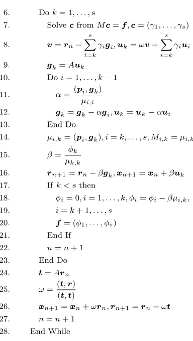
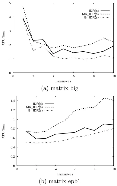
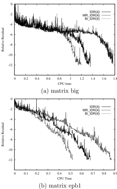
(4) Proceedings of the International MultiConference of Engineers and Computer Scientists 2009 Vol II IMECS 2009, March 18 - 20, 2009, Hong Kong. 6. 7.. Do k = 1, . . . , s. 8.. Solve c from M c = f , c = (γ1 , . . . , γs ) s s ∑ ∑ v = rn − γi g i , uk = ωv + γi ui. 9.. g k = Auk. i=k. i=k. 12.. Do i = 1, . . . , k − 1 (pi , g k ) α= µi,i g k = g k − αg i , uk = uk − αui. 13.. End Do. 14.. µi,k = (pi , g k ), i = k, . . . , s, Mi,k = µi,k. 15.. β=. 10. 11.. ϕk µk,k. 16.. r n+1 = r n − βg k , xn+1 = xn + βuk. 17.. If k < s then. 18.. ϕi = 0, i = 1, . . . , k, ϕi = ϕi − βµi,k ,. 19.. i = k + 1, . . . , s. 20.. f = (ϕ1 , . . . , ϕs ). 21.. End If. 22.. n=n+1. 23.. End Do. 24.. 26.. t = Ar n (t, r) ω= (t, t) xn+1 = xn + ωr n , r n+1 = r n − ωt. 27.. n=n+1. 25.. 28.. 5. End While. Numerical Experiments. In this section we discuss numerical experiments of IDR(s) method and MR IDR(s) method, Bi IDR(s) method. All computations are carried out in double precision floating-point arithmetic on a PC with a POWER5 processor (1.9GHz). Intel Fortran Compiler90 ver 7.1 and compile option -O3 -qtune=power5 -qarch=pw5 -qhot was used. In all cases the iteration was started with the initial guess solution x0 = 0. The maximum iterations was fixed as 10000. The value of s varies at the interval of 1 from 1 to 10. Twelve test matrices are from University of Florida Sparse Matrix Collection[1][3]. Description of test matrices is shown in Table 1. In this Table, ”nnz” means number of nonzero entries, and ”ave nnz” means number of nonzero entries per single row.. 5.1. Numerical Results. Table 2 shows iterations and CPU time in seconds of three iterative methods. In Table 2, ”sopt ” means optimum parameter s. CPU time is minimum at optimum parameter s. ”itr.” means number of iterations. ”ratio” means ratio of CPU time of each method to CPU time of IDR(s) method. The figure in bold means minimum CPU time of three iterative methods. From Table 2, the following observations can be made.. ISBN: 978-988-17012-7-5. Table 1: Description of test matrices. matrix dimension nnz ave nnz big 13,209 91,465 6.92 epb1 14,734 95,053 6.45 epb2 25,228 175,027 6.94 garon2 13,535 373,235 27.58 memplus 17,758 126,150 7.10 poisson3da 13,514 352,762 26.10 poisson3db 85,623 2,374,949 27.74 raefsky2 3,242 293,551 90.55 sme3da 12,504 874,887 69.97 sme3db 29,067 2,081,063 71.60 xenon1 48,600 1,181,120 24.30 xenon2 157,464 3,866,688 24.56. 1. Bi IDR(s) method converges fastest for 10 matrices. 2. CPU time of all methods are fastest at s = 3 for matrix epb1. 3. Iterations of MR IDR(s) method is minimum and that of Bi IDR(s) method is maximum for matrix epb1. 4. CPU time of Bi IDR(s) method is minimum and that of MR IDR(s) method is maximum for matrix epb1.. From the second and third, fourth observations you can see that computational cost of Bi IDR(s) method is minimum and that of MR IDR(s) method is maximum. Fig. 1 displays variation of iterations of three iterative methods for matrices big and epb1. In Fig. 1, we show variation of iterations of IDR(s) method in solid line and MR IDR(s) method in dashed line and Bi IDR(s) method in dotted line. From Fig. 1 you can see that iterations of MR IDR(s) method is minimum and that of IDR(s) method is maximum for almost cases. Fig. 2 shows variation of CPU time of three iterative methods for matrices big and epb1. From Fig. 2 you can see that CPU time of Bi IDR(s) method is minimum and that of MR IDR(s) method is maximum for almost cases. Fig. 3 plots relative residual of three iterative methods for matrices big and epb1. From Fig. 3 you can see that Bi IDR(s) method converges fastest and MR IDR(s) method converges slowest, and oscillation of relative residual norms of MR IDR(s) and Bi IDR(s) methods is more gentle than that of IDR(s) method.. IMECS 2009.

(5) Proceedings of the International MultiConference of Engineers and Computer Scientists 2009 Vol II IMECS 2009, March 18 - 20, 2009, Hong Kong. 7000. Table 2: Iterations and CPU time in seconds of three iterative methods.. IDR(s) MR_IDR(s) Bi_IDR(s). 6000. matrix. Iterations. 5000. time. 4000. 1000 0 0. 2. 4. 6. 8. 10. Parameter s. (a) matrix big 1200 IDR(s) MR_IDR(s) Bi_IDR(s). 1000. 800 CPU Time. IDR(s) MR IDR(s) Bi IDR(s) IDR(s) epb1 MR IDR(s) Bi IDR(s) IDR(s) epb2 MR IDR(s) Bi IDR(s) IDR(s) garon2 MR IDR(s) Bi IDR(s) IDR(s) memplus MR IDR(s) Bi IDR(s) poissonIDR(s) 3da MR IDR(s) Bi IDR(s) poissonIDR(s) 3db MR IDR(s) Bi IDR(s) IDR(s) raefsky2 MR IDR(s) Bi IDR(s) IDR(s) sme3da MR IDR(s) Bi IDR(s) IDR(s) sme3db MR IDR(s) Bi IDR(s) IDR(s) xenon1 MR IDR(s) Bi IDR(s) IDR(s) xenon2 MR IDR(s) Bi IDR(s) big. 3000 2000. 600. 400. 200. 0 0. 2. 4. 6. 8. 10. Parameter s. (b) matrix epb1 Figure 1: Variation of iterations of three iterative methods. 5 IDR(s) MR_IDR(s) Bi_IDR(s). 4. CPU Time. method sopt. itr.. 3. 2. 1. 4 4 7 2 2 2 3 2 2 2 3 2 5 3 2 2 4 4 5 3 5 7 3 7 7 9 7 9 6 4 2 3 4 1 1 1. 1687 1489 1111 818 803 833 450 473 481 777 722 758 574 751 782 263 232 238 528 551 518 420 491 431 2272 2088 2415 2668 3441 3546 2240 2015 1952 2725 2847 2911. 1.36 1.77 0.98 0.58 0.72 0.49 0.68 0.79 0.54 1.26 1.31 1.12 0.67 0.95 0.62 0.52 0.54 0.46 15.31 16.00 14.77 0.40 0.44 0.38 9.30 10.01 9.59 45.47 56.62 44.53 12.12 12.98 10.74 77.89 84.88 78.01. ratio [sec.] 1.00 1.30 0.72 1.00 1.24 0.84 1.00 1.16 0.79 1.00 1.04 0.89 1.00 1.42 0.93 1.00 1.04 0.88 1.00 1.05 0.96 1.00 1.10 0.95 1.00 1.08 1.03 1.00 1.25 0.98 1.00 1.07 0.89 1.00 1.09 1.00. mem. [MB] 2.91 3.82 3.92 2.49 3.06 2.61 4.99 5.37 4.60 5.76 6.07 5.86 4.36 4.49 3.27 5.33 6.87 6.05 41.22 41.88 41.88 4.05 3.92 4.07 12.64 15.02 12.73 31.25 32.13 28.14 18.15 21.86 20.75 55.66 59.27 56.87. 0 0. 2. 4. 6. 8. 10. Parameter s. (a) matrix big. 5.2. 1.4 IDR(s) MR_IDR(s) Bi_IDR(s). 1.2. The solution vector of IDR(s) method sometime isn’t accurate when value of s is large. Thereby, we inspect the accuracy of the solution vector of MR IDR(s) and Bi IDR(s) method. Test matrix is real unsymmetric Toeplitz matrix. Number of columns of Toeplitz matrix is 2000, and parameter γ is 1.5.. 1 CPU Time. Verification of the solution vector with degraded accuracy. 0.8 0.6 0.4 0.2 0 0. 2. 4. 6. 8. 10. Parameter s. (b) matrix epb1 Figure 2: Variation of CPU Time of three iterative methods.. ISBN: 978-988-17012-7-5. Fig. 4 draws variation of common logarithm of TRR(true relative residual) 2-norm of four iterative methods for matrix Toeplitz. In Fig. 4, TRR 2-norm is defined by ||b − Axn ||2 /||b − Ax0 ||2 . We show variation of TRR of IDR(s) method in solid line, and IDR(s) method with the additional operation for parameter ω in chained line , MR IDR(s) method in dashed line , Bi IDR(s) method in. IMECS 2009.

(6) Proceedings of the International MultiConference of Engineers and Computer Scientists 2009 Vol II IMECS 2009, March 18 - 20, 2009, Hong Kong. 0. 0 IDR(4) MR_IDR(4) Bi_IDR(4). -2. IDR(s) IDR(s), k = 0.7 MRIDR(s) BiIDR(s). -2 -4. -6. -6 TRR. Relative Residual. -4. -8. -8. -10. -10. -12. 0. 0.2. 0.4. 0.6. 0.8 1 CPU time. 1.2. 1.4. 1.6. 1.8. (a) matrix big. -12. 0. IDR(4) MR_IDR(4) Bi_IDR(4). -2. 20. 30. 40. 50. Figure 4: Variation of True Relative Residual 2-norm of four iterative methods for matrix Toeplitz.. -4 Relative Residual. 10. Parameter s. 0. -6 -8. References. -10 -12. 0. 0.1. 0.2. 0.3. 0.4 0.5 CPU Time. 0.6. 0.7. 0.8. 0.9. (b) matrix epb1 Figure 3: Relative residual history of three iterative methods.. [1] Davis, T. : Univ. of Florida sparse matrix collection, http://www.cise.ufl.edu/research/sparse/matrices /index.html [2] H. A. van der Vorst: Iterative Krylov preconditionings for large linear systems, Cambridge University Press, (2003). [3] Webpage of Matrix Market: http://math.nist.gov/ MatrixMarket/matrices.html. dotted line. We set parameter κ for the additional computation as κ = 0.7, because the κ = 0.7 is recommended by Sleijpen and van der Vorst[4]. From Fig. 4, you can see that the accuracy of IDR(s) improves if the additional operation for parameter ω is adopted, and the solution vector of MR IDR(s) and Bi IDR(s) methods is more accurate than that of IDR(s) method.. 6. Concluding Remarks. We overviewed MR IDR(s) and Bi IDR(s) methods based on IDR Theorem. Next, we evaluated performance of these methods through numerical experiments. As a result, we concluded that MR IDR(s) method converges slower than original IDR(s) method because of high cost of evaluating intermediate residua norm. On the other hand, Bi IDR(s) method converges faster than original IDR(s) method because of low computational cost. Furthermore, MR IDR(s) and Bi IDR(s) methods clearly improve the accuracy of original IDR(s) method.. ISBN: 978-988-17012-7-5. [4] Sleijpen, G., van der Vorst, H.: Maintaining convergence properties of BiCGstab methods in finite precision arithmetic, Numerical Algorithms, Vol.10, pp.203-223, 1995. [5] Sonneveld, P., van Gijzen, M.B.: IDR(s): a family of simple and fast algorithms for solving large nonsymmetric linear systems, TR 07-07, Delft Univ. of Tech., 2007. [6] van Gijzen, M.B., Sonneveld, P.: An elegant IDR(s) variant that efficiently exploits bi-orthogonality properties, TR 08-21, Delft Univ. of Tech., 2008. [7] van Gijzen, M.B., Sonneveld, P.: An IDR(s) variant with minimal intermediate residual norms, The Proc. of Int. Kyoto-Forum on Krylov Subspace method, pp.85-92, 2008. [8] Wesseling, P., Sonneveld, P.: Numerical Experiments with a Multiple Grid- and a Preconditioned Lanczos Type Methods, Lecture Notes in Math., Springer, No.771, pp.543-562, 1980.. IMECS 2009.

(7)

No results found