Web-Scale Language-Independent Cataloging of Noisy Product Listings
for E-Commerce
Pradipto Das, Yandi Xia, Aaron Levine, Giuseppe Di Fabbrizio, and Ankur Datta
Rakuten Institute of Technology, Boston, MA, 02110 - USA
{pradipto.das, ts-yandi.xia, aaron.levine}@rakuten.com
{giuseppe.difabbrizio, ankur.datta}@rakuten.com
Abstract
The cataloging of product listings through taxonomy categorization is a fundamental problem for any e-commerce marketplace, with applications ranging from personal-ized search recommendations to query un-derstanding. However, manual and rule based approaches to categorization are not scalable. In this paper, we compare sev-eral classifiers for categorizing listings in both English and Japanese product cata-logs. We show empirically that a
combina-tion of words from product titles,
naviga-tional breadcrumbs, andlist prices, when
available, improves results significantly. We outline a novel method using corre-spondence topic models and a lightweight manual process to reduce noise from mis-labeled data in the training set. We con-trast linear models, gradient boosted trees (GBTs) and convolutional neural networks (CNNs), and show that GBTs and CNNs yield the highest gains in error reduc-tion. Finally, we show GBTs applied in a language-agnostic way on a large-scale Japanese e-commerce dataset have improved taxonomy categorization perfor-mance over current state-of-the-art based on deep belief network models.
1 Introduction
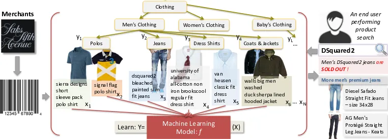
Web-scale e-commerce catalogs are typically ex-posed to potential buyers using a taxonomy cat-egorization approach where each product is cate-gorized by a label from the taxonomy tree. Most e-commerce search engines use taxonomy labels to optimize query results and match relevant list-ings to users’ preferences (Ganti et al., 2010). To illustrate the general concept, consider Fig. 1. A merchant pushes new men’s clothing listings to
an online catalog infrastructure, which then orga-nizes the listings into a taxonomy tree. When a
user searches for a denim brand, “DSquared2”,
the search engine first has to understand that the
user is searching for items in the“Jeans”category.
Then, if the specific items cannot be found in the
inventory, other relevant items in the “Jeans”
cat-egory are returned in the search results to encour-age the user to browse further. However, achiev-ing good product categorization for e-commerce market-places is challenging.
Commercial product taxonomies are organized in tree structures three to ten levels deep, with thousands of leaf nodes (Sun et al., 2014; Shen et al., 2012b; Pyo et al., 2016; McAuley et al., 2015). Unavoidable human errors creep in while upload-ing data usupload-ing such large taxonomies, contributupload-ing to mis-labeled listing noise in the data set. Even EBay, where merchants have a unified taxonomy,
reported a15%error rate in categorization (Shen
et al., 2012b). Furthermore, most e-commerce companies receive millions of new listings per month from hundreds of merchants composed of wildly different formats, descriptions, prices and
meta-data for the same products. For instance,
the two listings,“University of Alabama all-cotton
non iron dress shirt” and “U of Alabama 100%
cotton no-iron regular fit shirt”by two merchants
refer to the same product.
E-commerce systems trade-off between classi-fying a listing directly into one of thousands of
leaf node categories (Sun et al., 2014; ?) and
splitting the taxonomy at predefined depths (Shen
et al., 2011; ?) with smaller subtree models. In
the latter case, there is another trade-off between the number of hierarchical subtrees and the prop-agation of error in the prediction cascade. Simi-lar to (Shen et al., 2012b; Cevahir and Murakami, 2016), we classify product listings in two or three steps, depending on the taxonomy size. First, we predict the top-level category and then
(X) Learn: Y=
Men’s Clothing
Polos Jeans Dress Shirts Coats & Jackets …
Machine Learning
Model: f
sierra designs short sleeve pack polo shirt
signal flag polo shirt
dsquared2 bleached painted slim fit jeans
university of alabama all-cotton non iron brookscool regular fit dress shirt
walls big men washed duck sherpa lined hooded jacket … x1
x2 x3
x4 x6
y1 y2 y3 y4 yL
xN
DSquared2
Diesel Safado Straight Fit Jeans – size 34x28
AG Men's Protégé Straight Leg Jeans - Keats
Men’s DSquared2 jeansare
SOLD OUT !
More men’s premium jeans
Merchants An end user
performing product
search Women’s Clothing Baby’s Clothing
Clothing
[image:2.595.107.488.51.188.2]van heusen classic fit dress shirt x5
Figure 1: E-commerce platform using taxonomy categorization to understand query intent, match
mer-chant listings to potential buyers as well as to prevent buyers from navigating away on search misses.
sify the listings using another one or two levels of subtree models selected by the previous predic-tions. For our large-scale taxonomy categoriza-tion experiments on product listings, we use two
in-house datasets,1 a publicly available Amazon
product dataset (McAuley et al., 2015), and a
pub-licly available Japanese product dataset.2
Our paper makes several contributions: 1) We perform large-scale comparisons with several ro-bust classification methods and show that
Gradi-ent Boosted Trees (GBTs) (Friedman, 2000; ?)
and Convolutional Neural Networks (CNNs)
(Le-Cun and Bengio, 1995; ?) perform substantially
better than state-of-the-art linear models (Section 5). We further provide analysis of their perfor-mance with regards to imbalance in our datasets.
2) We demonstrate that using both listing price
andnavigational breadcrumbs– the branches that
merchants assign to the listings in web pages for navigational purposes – boost categorization per-formance (Section 5.3). 3) We effectively apply correspondence topic models to detect and remove mis-labeled instances in training data with mini-mal human intervention (Section 5.4). 4) We em-pirically demonstrate the effectiveness of GBTs on a large-scale Japanese product dataset over a re-cently published state-of-the-art method (Cevahir and Murakami, 2016), and in turn the otherwise language-agnostic capabilities of our system given a language-dependent word tokenization method. 2 Related Work
The nature of our problem is similar to those re-ported in (Bekkerman and Gavish, 2011; Shen et al., 2011; Shen et al., 2012b; Yu et al., 2013b;
Sun et al., 2014; Kozareva, 2015; ?), but with
1The in-house datasets are from Rakuten USA, managed
by Rakuten Ichiba, Japan’s largest e-commerce company.
2This dataset is from Rakuten Ichiba and is released under
Rakuten Data Release program.
more pronounced data quality issues. However, the existing methods for noisy product classifica-tion have only been applied to English. Their
effi-cacy formoraicandagglutinativelanguages such
as Japanese remains unknown.
The work in Sun et al. (2014) emphasizes the use of simple classifiers in combination with large-scale manual efforts to reduce noise and imperfec-tions from categorization outputs. While human intervention is important, we show how unsuper-vised topic models can substantially reduce such expensive efforts for product listings crawled in the wild. Further, unlike Sun et al. (2014), we adopt stronger baseline systems based on regu-larized linear models (Hastie et al., 2003; Zhang, 2004; Zou and Hastie, 2005).
A recent work from Pyo et al. (2016) empha-sizes the use of recurrent neural networks for tax-onomy categorization purposes. Although, they mention that RNNs render unlabeled pre-training of word vectors (Mikolov et al., 2013) unneces-sary, in contrast, we show that training word em-beddings on the whole set of three product title corpora improves performance for CNN models and opens up the possibility of leveraging other product corpora when available.
Shen et al. (2012b) advocate the use of algorith-mic splitting of the taxonomy using graph theo-retic latent group discovery to mitigate data imbal-ance problems at the leaf nodes. They use a com-bination of k-NN classifiers at the coarser level and SVMs (Cortes and Vapnik, 1995) classifiers at the leaf levels. Their SVMs solve much easier
k-way multi-class categorization problems where
k∈ {3,4,5}with much less data imbalance. We,
however, have found that SVMs do not work well
in scenarios where kis large and the data is
prohibitively long prediction times under arbitrary feature transformations (Manning et al., 2008; Ce-vahir and Murakami, 2016).
The use of a bi-level classification using k-NN and hierarchical clustering is incorporated in Ce-vahir and Murakami (2016)’s work, where they use nearest neighbor methods in addition to Deep Belief Networks (DBN) and Deep Auto Encoders (DAE) over both titles and descriptions of the Japanese product listing dataset. We show in Sec-tion 5.6, that using a tri-level cascade of GBT clas-sifiers over titles, we significantly outperform the k-NN+DBN classifier on average.
3 Dataset Characteristics
We use two in-house datasets, named BU1 and BU2, one publicly available Amazon dataset (AMZ) (McAuley et al., 2015), and a Japanese product listing dataset named RAI (Cevahir and Murakami, 2016) (short for Rakuten Ichiba) for the experiments in this paper.
BU1 is categorized using human annotation ef-forts and rule-based automated systems. This leads to a high precision training set at the expense of coverage. On the other hand, for BU2, noisy taxonomy labels from external data vendors have been automatically mapped to an in-house taxon-omy without any human error correction, resulting in a larger dataset at the cost of precision. BU2 also suffers from inconsistencies in regards to in-complete or malformed product titles and meta-data arising out of errors in the web crawlers that vendors use to aggregate new listings. However, for BU2, the noise is distributed identically in the training and test sets, thus evaluation of the classi-fiers is not impeded by it.
The Japanese RAI dataset consists of
172,480,000 records split across 26,223
leaf nodes. The distribution of product listings in the leaf nodes is based on the popularity of certain product categories and is thus highly imbalanced. For instance, the top level “Sports & Outdoor”
category has 2,565leaf nodes, while the “Travel
/ Tours / Tickets” category has only38. The RAI
dataset has 35 categories at depth one (level-one
categories) and400categories at depth two of the
full taxonomy tree. The total depth of the tree varies from three to five levels.
The severity of data imbalance for BU2 is
shown in Figure 2. The top-level“Home,
Furni-ture and Patio” subtree that accounts for almost
half of the BU2 dataset. Table 1 shows dataset
0 1 2 3 4 5 6 7 8 9 10 11 12 13 14 15
Mi
lli
on
s Toys Home, Furniture and Pa]o
Jewelry Watches Bag, Handbags and Accessories Health, Beauty and Fragrance Shoes
Electronics and Computers Office
[image:3.595.319.510.62.192.2]Sports Fitness Automo]ve Industrial Baby Products Baby Kids Clothes Men's Clothing Women's Clothing
Figure 2: Top-level category distribution of 40
million deduplicated listings from an earlier Dec 2015 snapshot of BU2. Each category subtree is also imbalanced, as seen in exploded view of the
“Home, Furniture, and Patio”category.
characteristics for the four different kinds of prod-uct datasets we use in our analyses. It lists the number of branches for the top-level taxonomy subtrees, the total number of branches ending at leaf nodes for which there are a non-zero num-ber of listings and two important summary statis-tics that helps quantify the nature of imbalance. We first calculate the Pearson correlation coeffi-cient (PCC) between the number of listings and branches in each of the top-level subtrees for each of the four datasets.
A perfectly balanced tree will have a PCC of
1.0. BU1 shows the mostbenign kind of
imbal-ance with a PCC of 0.643. This confirms that
the number of branches in the subtrees correlate well with the volume of listings. Both AMZ and RAI datasets show the highest branching factors in their taxonomies. For the AMZ dataset, it could be
Datasets Subtrees Branches Listings PCC KL
BU1 16 1,146 12.1M 0.643 0.872
BU2 15 571 60M 0.209 0.715
AMZ 25 18,188 7.46M 0.269 1.654
RAI 35 26,223 172.5M 0.474 7.887
Table 1: Dataset properties on: total number of
top-level category subtrees, branches and listings due to the fact that the crawled taxonomy is differ-ent from Amazon’s internal catalog. The Rakuten Ichiba taxonomy has been incrementally adjusted to grow in size over several years by creating new branches to support newer and popular products. We observe that for RAI, AMZ and BU2 in par-ticular, the number of branches in the subtrees do not correlate well with the volume of listings. This indicates a much higher level of imbalance.
[image:3.595.306.532.526.589.2](KL) divergence, KL(p(x)|q(x)), (Cover and Thomas, 1991) between the empirical distribution over listings in branches for each subtree rooted in
the nodes at depth one,p(x), compared to a
uni-form distribution,q(x). Here, the KL divergence
acts as a measure of imbalance of the listing distri-bution and is indicative of the categorization per-formance that one may obtain on a dataset; high KL divergence leads to poorer categorization and vice-versa (see Section 5).
4 Gradient Boosted Trees and Convolutional Neural Networks
GBTs (Friedman, 2000) optimize a loss
func-tional: L = Ey[L(y, F(x)|X)] whereF(x) can
be a mathematically difficult to characterize
func-tion, such as a decision tree f(x) over X. The
optimal value of the function is expressed as
F?(x) = PM
m=0fm(x,a,w), wheref0(x,a,w)
is the initial guess and{fm(x,a,w)}Mm=1are
ad-ditive boosts on x defined by the optimization
method. The parameter am of fm(x,a,w)
de-notes split points of predictor variables and wm
denotes the boosting weights on the leaf nodes of the decision trees corresponding to the partitioned
training set Xj for regionj. To compute F?(x),
we need to calculate, for each boosting roundm,
{am,wm}= arg mina,w
N X
i=1
L(yi, Fm(xi)) (1)
withFm(x) = Fm−1(x) +fm(x,am,wm). This
expression is indicative of a gradient descent step:
Fm(x) =Fm−1(x) +ρm(−gm(xi)) (2)
where ρm is the step length and
h
∂L(y,F(x)) ∂F(x)
i
F(xi)=Fm−1(xi) = gm(xi) being the
search direction. To solveam andwm, we make
the basis functions fm(xi;a,w) correlate most
to−gm(xi), where the gradients are defined over
thetraining datadistribution. In particular, using
Taylor series expansion, we can get closed form
solutions foramandwm– see Chen and Guestrin
(2016) for details. It can be shown that am =
arg minaPNi=1(−gm(xi)−ρmfm(xi,a,wm))2
and ρm = arg minρPNi=1L(yi, Fm−1(xi) +
ρfm(xi;am,wm))which yields,
Fm(x) =Fm−1(x) +ρmfm(x,am,wm) (3)
Each boosting round m updates the weights
wm,j on the leaves and helps create a new tree
in the next iteration. The optimal selection of de-cision tree parameters is based on optimizing the
fm(x,a,w)using a logistic loss. For GBTs, each
decision tree is resistant to imbalance and outliers
(Hastie et al., 2003), andF(x) can approximate
arbitrarily complex decision boundaries.
The convolutional neural network we use is based on the CNN architecture described in Le-Cun and Bengio (1995; Kim (2014) using the Ten-sorFlow framework (Abadi and others, 2015). As in Kim (2014), we enhance the performance of
“vanilla” CNNs (Fig. 3 right) using word
em-bedding vectors (Mikolov et al., 2013) trained on the product titles from all datasets, without
taxon-omy labels. Context windows of width n,
corre-sponding to n-grams and embedded in a 300
di-mensional word embedding space, are convolved
withLfilters followed by rectified non-linear unit
activation and a max-pooling operation over the
set of all windowsW. This operation results in a
L×1vector, which is then connected to a softmax
output layer of dimensionK×1, whereK is the
number of classes. Section A lists more details on parameters.
The CNN model tries to allocate as few filters to the context windows while balancing the con-straints on the back-propagation of error
resid-uals with regards to cross-entropy loss L =
−PKk=1qklogpk, wherepk is the probability of
a product titlexbelonging to classkpredicted by
our model, andq ∈ {0,1}K is a one-hot vector
that represents the true label of title x. This
re-sults in a higher predictive power for the CNNs, while still matching complex decision boundaries in a smoother fashion than GBTs. We note here that for all models, the predicted probabilities are
notcalibrated (Zadrozny and Elkan, 2002).
5 Experimental Setup and Results
We use Na¨ıve Bayes (NB) (Ng and Jordan, 2001) similar to the approach described in Shen et al. (2012a) and Sun et al. (2014), and Logistic
Re-gression (LogReg) classifiers withL1 (Fan et al.,
2008) and Elastic Net regularization, as robust baselines. Parameter setups for the various models and algorithms are mentioned in Section A. 5.1 Data Preprocessing
Product listing datasets in English– BU1 is
65.00 70.00 75.00 80.00 85.00 90.00 95.00 100.00 ap par el & ac ce ss or ie s ap pl ian ce s au to m ot iv e ba by pr oduc ts el ec tr on ic s & a cc es so ries gr oc er y & go ur m et fo od he al th & be aut y ho m e & k itc he n je w el ry & w at che s of fic e pr od uc ts pe t s uppl ie s sh oe s sp or ts & o ut do or s tic ke ts & e ve nts to ol s & h om e im pr ov em en t to ys & g am es
NB LogReg ElasticNet (OvA) LogReg L1 (OvO) GBT
CNN w/ pretraining CNN-Vanilla
78 80 82 84 86 88 90 Word Unigram Count Word Unigram BiPosi9onal Count Word Bigram Count Word Bigram BiPosi9onal Count NB LogReg Elas9cNet (OvA) LogReg L1 (OvO) GBT
[image:5.595.78.520.61.209.2]CNN w/ pretraining CNN vanilla
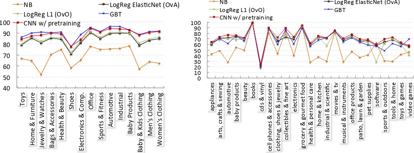
Figure 3: Classifier performance on BU1 test set. The CNN classifier has only one configuration and
thus shows constant curves in all plots.Leftfigure shows prediction on10% test set using word unigram
count features; middlefigure shows prediction on10% test set using word bigram bi-positional count
features; and therightfigure shows mean micro-precision over different feature setups except CNNs. In
all figures, “OvO” means “One vs. One” and “OvA” means “One vs All”.
price whenever available. For BU2, we also use
the leaf node of any availablenavigational
bread-crumbs. In order to decrease training and cate-gorization run times, we employ a number of vo-cabulary filtering methods. Further, English
stop-words and rare tokens that appear in 10 listings
or less are then filtered out. This reduces
vocabu-lary sizes by up to 50%, without a significant
re-duction in categorization performance. For CNNs,
we replace numbers by the nominal form[NUM]
and remove rare tokens. We also remove punctua-tions and then lowercase the resulting text. Parts of speech (POS) tagging using a generic tagger from Manning et al. (2014) trained on English text pro-duced very noisy features, as is expected for out-of-domain tagging. Consequently, we do not use POS features due to the absence of a suitable train-ing set for listtrain-ings unlike that in Putthividhya and Hu (2011). For GBTs, we also experiment with title word expansion using nearest neighbors from Word2Vec model (Mikolov et al., 2013), for
in-stance, to group words like “t-shirts”, “tshirt”,
“t-shirt” in their respective equivalence classes,
however, the overall results have not been better.
Product listing datasets in Japanese – CJK
languages like Japanese lack white space between words. Hence, the first pprocessing step re-quires a specific Japanese tokenization tool to properly segment the words in the product titles.
For our experiments, we used the MeCab3
to-kenizer trained using features that are augmented with in-house product keyword dictionaries. Ro-maji words written using Latin characters are
sep-3https://sourceforge.net/projects/mecab/
arated from Kanji and Kana words. All brack-ets are normalized to square brackbrack-ets and punc-tuations from non-numeric tokens are removed. We also use canonical normalization to change the code points of the resulting Japanese text into
an NFKC normalized4 form, then remove
any-thing outside of standard Japanese UTF-8 charac-ter ranges. Finally, the resulting text is lowercased. Due to the size of the RAI dataset taxonomy tree, three groups of models are trained to
clas-sify new listings into one of 35 level-one
cate-gories, then one of400level-two categories, and,
finally, the leaf node of the taxonomy tree. We have found this scheme to be working better for the RAI dataset than a bi-level scheme that we adopted for the other English datasets.
Applying GBTs on the Japanese dataset in-volved a bit more feature engineering. At the to-kenized word-level, we use counts of word uni-grams and word bi-uni-grams. For character features, the product title is first normalized as discussed
above. Consequently, character2,3, and4-grams
are extracted with their counts, where extractions include single spaces appearing at the end of word boundaries. Identification of the best set of fea-ture combinations in this case has been performed during cross-validation.
5.2 Initial Experiments on BU1 dataset Our initial experiments use unigram counts and three other features: word bigram counts, positional unigram counts, and positional
bi-gram counts. Consider a title text “120 gb hdd
5400rpm sata fdb 2 5 mobile” from the “Data
storage” leaf node of the Electronics taxonomy
subtree and another title text “acer aspire v7
582pg 6421 touchscreen ultrabook 15 6 full hd in-tel i5 4200u 8gb ram 120 gb hdd ssd nvidia geforce
gt 720m”from the “Laptops and notbooks”leaf
node. In such cases, we observe that merchants tend to place terms pertaining to storage device
specifics in the front of product titles for “Data
storage”and similar terms towards the end of the
titles for “Laptops”. As such, we split the title
length in half and augment word uni/bigrams with a left/right-half position.
This makes sense from a Na¨ıve Bayes point
of view, since terms like “120 gb”[Left Half],
“gb hdd”[Left Half], “120 gb”[Right Half] and
“gb hdd”[Right Half] de-correlates the feature space better, which is suitable for the na¨ıve as-sumption in NB classification. This also helps in sightly better explanation of the class posteri-ors. These assumptions for NB are validated in the
three figures: Fig. 3left, Fig. 3 middleand Fig.
3 right. Word unigram count features perform
strongly for all classifiers except NB, whereas bi-positional word bigram features helped only NB significantly.
Additionally, the micro-precision and F1 scores for CNNs and GBTs are significantly higher com-pared to other algorithms on word unigrams using
paired t-test with a p-value< 0.0001. The
per-formances of GBTs and LogRegL1classifiers
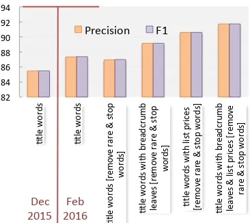
de-teriorate over the other feature sets as well. The bi-positional and bigram feature sets also do not produce any improvements for the AMZ dataset. Based on these initial results, we focus on word unigrams in all of our subsequent experiments. 5.3 Categorization Improvements with
Navigational Breadcrumbs and List Prices on BU2 Dataset
BU2 is a challenging dataset in terms of class im-balance and noise and we sought to improve cate-gorization performance using available meta-data. To start, we experiment with a smaller dataset
con-sisting of≈ 500,000deduplicated listings under
the “Women’s Clothing” taxonomy subtree,
ex-tracted from our Dec 2015 snapshot of40million
records. Then we train and test against ≈ 2.85
million deduplicated“Women’s Clothing”listings
from the Feb 2016 snapshot of BU2. In all
exper-iments, 10% of the data is used as test set. The
womens clothing category had been chosen due to the importance of the category from a business
82 84 86 88 90 92 94
]tl
e
w
or
ds
]tl
e
w
or
ds
]tl
e
w
or
ds
[r
em
ov
e
rar
e
&
s
to
p
wo
rd
s]
]tl
e
w
or
ds
w
ith
b
re
ad
cr
um
b
le
av
es
[r
em
ov
e
rar
e
&
s
to
p
wo
rd
s]
]tl
e
w
or
ds
w
ith
li
st
pr
ic
es
[r
em
ov
e
rar
e
&
s
to
p
w
or
ds
]
]tl
e
w
or
ds
w
ith
b
re
ad
cr
um
b
le
av
es
&
li
st
pr
ic
es
[r
em
ov
e
rar
e
&
s
to
p
w
or
ds
]
Precision F1
[image:6.595.323.506.59.222.2]Dec 2015 2016 Feb
Figure 4: Improvements in micro-precision and
F1 for GBTs on BU2 dataset for“Women’s
Cloth-ing”subtree
standpoint, which provided early access to listings in this category. Further, data distributions remain the same in the two snapshots and the Feb 2016 snapshot consists of listings in addition to those for the Dec 2015 snapshot.
The first noteworthy fact in Fig. 4 is that the micro-precision and F1 of the GBTs substantially improve after increasing the size of the dataset. Further, stop words and rare words filtering
de-crease precision and F1 by less than1%, despite
halving the feature space. The addition of navi-gational leaf nodes and list prices prove advanta-geous, with both features independently boosting performance and raising micro-precision and F1 to
over90%. Despite finding similar gains in
catego-rization performance for other top-level subtrees by using these meta features, we needed a system to filter mis-categorized listings from our training data as well.
5.4 Noise Analysis of BU2 Dataset using Correspondence LDA for Text
The BU2 dataset has the noisiest ground-truth la-bels, as incorrect labels have been assigned to product listings. However, since the manual ver-ification of millions of listings is infeasible, using some proxy for ground truth is a viable alternative that has previously produced encouraging results (Shen et al., 2012b). We next describe how resort-ing to unsupervised topic models helped to detect and remove incorrect listings.
As shown in Fig. 8, categorization
perfor-mance for the “Shoes”taxonomy subtree is over
25 points below the “Women’s Clothing”
cat-hardcover guide design handbook international health
business social law
heart diamond pearl 40 ring sterling chain charm 39 14k 47
paperback book history god home und soul stories journey bible der vhs world series
time king war ball house trek christmas space
i c love day e night u single lady child woman uk good
deluxe park
set 20 100 24 case kit oz 30 hand drive body wall digital ft
48 spray paper license standard
symantec system service cisco support year
dvd jazz media mixed country artists vol play music product pop
de calendar la american disc el 2013 art 2009 ray
[image:7.595.308.506.62.170.2]2012 compact
Figure 5: Selection of most probable
words under the latent “noise” topics over
listings in“Shoes”subtree. Human
anno-tators inspect whether such sets of words belong to a Shoes topic or not.
oxford burgundy plain
espresso wing madison Oxfords > Men’s Shoes > Shoes pr boots work mens blk
composite Boots > Men’s Shoes > Shoes tan polyurethane life
saddle stride bed Flats > Women’s Shoes > Shoes 13 reac]on york ak
driving steven Sneakers & Athle]c Shoes > Men’s Shoes > Shoes original rose bone mark
lizard copper Climbing > Men’s Shoes > Shoes
[image:7.595.96.275.64.172.2]Ambiguous labels
Figure 6: Interpretation of latent topics
us-ing predictions from a GBT classifier. The topics here do not include those in Fig. 5, but are all from Feb 2016 snapshot of the BU2 dataset.
egories. However, unlike Sun et al. (2014), as
there are over3.4million“Shoes” listings in the
BU2 dataset, a manual analysis to detect noisy la-bels is infeasible. To address this problem, we
computep(x)over latent topicszk, and
automati-cally annotate the most probable words over each topic.
We choose our CorrMMLDA model (Das et al., 2011) to discover the latent topical structure of the
listings in the “Shoes” category because of two
reasons. Firstly, the model is a natural choice for our scenario since it is intuitive to assume that store and brand names are distributions over words in titles. This is illustrated in the graphical model
in Fig. 7, where the store“Saks Fifth Avenue”and
the brand “Joie” are represented as words wd,m
in the M plate of listing d and are distributions
over the words in the product title“Joie kidmore
Embossed slipon sneakers”represented as words
wd,nin theN plate of the same listingd. The
ti-tle words are in turn distributions over the latent
topicszdfor listingd∈ {1..D}.
Secondly, the CorrMMLDA model has been shown to exhibit lower held-out perplexities in-dicative of improved topic quality. The reason be-hind the lower perplexity stems from the follow-ing observations: Usfollow-ing the notation in Das et al. (2011), we denote the free parameters of the vari-ational distributions over words in brand and store
names, sayλd,m,n, as multinomials over words in
the titles and those over words in the title, say
φd,n,k, as multinomials over latent topics zd. It
is easy to see that the posterior over the topiczd,k
for eachwd,mof brand and store names, is
depen-dent on λand φthrough PNd
n=1λd,m,n ×φd,n,k.
This means that if a certain topiczd = j
gener-ates all words in the title, i.e., φd,n,j > 0, then
wn
α zn r
β N
M ym wm
wdN=
D K
Joie Kidmore Embossed Slipon sneakers
wdM=
Saks Fifth Avenue Joie
Figure 7:Correspondence MMLDA model.
only that topic also generates the brand and store names thereby increasing likelihood of fit and
re-ducing perplexity. The other topicszd 6=jdo not
contribute towards explaining the topical structure
of the listingd.
60 65 70 75 80 85 90 95 100
Toy
s
Ho
m
e
&
F
ur
ni
tu
re
Je
w
el
ry
&
W
atc
he
s
Bag
s
&
A
cc
es
so
rie
s
He
al
th
&
B
eau
ty
Shoe
s
El
ec
tr
on
ic
s
&
C
om
p.
Offi
ce
Sp
or
ts
&
F
itn
es
s
Au
to
m
o]
ve
In
du
str
ial
Bab
y
Pr
od
uc
ts
Bab
y
&
K
id
s
Cl
oth
es
Me
n'
s
Cl
oth
in
g
W
om
en
's
C
lo
th
in
g
LOGREG L1 MICRO PRECISION LOGREG L1 MICRO F1
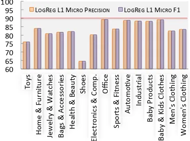
Figure 8: Micro-precision and F1 across fifteen
top-level categories on10% (4 million listings) of
Dec 2015 BU2 snapshot.
We train the CorrMMLDA model withK=100
latent topics. A sample of nine latent topics and their most probable words shown in Fig. 5
demon-strates that topics outside of the“Shoes”domain
can be manually identified, while reducing
hu-man annotation efforts from 3.4 million records
to one hundred. We choose K = 100 since it
[image:7.595.318.511.256.317.2] [image:7.595.322.509.431.570.2]40 50 60 70 80 90 100 Toy s Ho m e & F ur ni tu re Je w el ry & W atc he s Bag s & A cc es so rie s He al th & B eau ty Shoe s El ec tr on ic s & C om p. Offi ce Sp or ts & F itn es s Au to m oI ve In du str ial Bab y Pr od uc ts Bab y & K id s Cl oth in g Me n' s Cl oth in g W om en 's C lo th in g
NB LogReg ElasIcNet (OvA) LogReg L1 (OvO) GBT
[image:8.595.92.505.65.218.2]CNN w/ pretraining
Figure 9: Micro-precision on 10% of
BU2 across categories (see Sect. 5.4)
0 10 20 30 40 50 60 70 80 90 100 ap pl ian ce s ar ts , c ra7 s & s ew in g au to m o> ve bab y pr od uc ts be au ty book s cd
s & vi
nyl ce ll ph on es & ac ce ss or ie s cl oth in g, s ho es & je w el ry co lle c> bl es & fi ne ar t el ec tr on ic s gr oc er y & g ou rm et fo od he al th & p er so nal c ar e ho m e & k itc he n in du str ial & s ci en >fi c m ov ie s & tv m us ic al & in str um en ts offi ce p ro du cts pa> o, law n & g ar de n pe t s up pl ie s so 7 w ar e sp or ts & o utd oo rs to ol s & h om e to ys & g am es vi de o gam es
NB LogReg Elas>cNet (OvA)
LogReg L1 (OvO) GBT
CNN w/ pretraining
Figure 10:Micro-precision on10% of AMZ across
categories
Dataset NB LogReg ElasticNet LogReg L1 GBT CNN w pretraining Mean KL log(N/B)
BU1 81.45 86.30 86.75 89.03* 89.12* 0.872 9.27
BU2 68.21 84.29 85.01 90.63* 88.67 0.715 11.54
[image:8.595.85.509.263.311.2]AMZ 49.01 69.39 66.65 67.17 72.66* 1.654 6.02
Table 2: Mean micro-precision on10% test set from BU1, BU2 and AMZ English datasets
truth classes.
We next run a list of the most probable six
words, the average length of a“Shoes”listing’s
ti-tle, from each latent topic through our GBT
classi-fier trained on the full, noisy data,but without
con-sidering any metadata, due to bag-of-words nature of the topic descriptions. As shown in the bottom two rows in Fig. 6, categories mismatching their topics are manually labeled as ambiguous. As a fi-nal validation, we uniformly sampled a hundred listings from each ambiguous topic detected by the model. Manual inspections revealed numer-ous listings from merchants not selling shoes are
wrongly cataloged in the“Shoes” subtree due to
vendor’s error. To this end, we remove listings
cor-responding to such “out-of-category” merchants
from all top-level categories.
Thus, by manually inspectingK×6most
prob-able words from theK=100topics and J ×100
listings, whereJ << K, instead of3.4million, a
few annotators accomplished in hours what would have taken hundreds of annotators several months according to the estimates in Sun et al. (2014). 5.5 Results on BU2 and AMZ Datasets In section 5.2, we have shown the efficacy of word unigram features on the BU1 dataset. Figure 8
shows that LogReg with L1 regularization (Yu
et al., 2013b; Yu et al., 2013a) initially achieves 83% mean micro-precision and F1 on the initial BU2 dataset. This falls short of our expectation
of achieving an overall90% precision (red line in
Fig. 8), but forms a robust baseline for our subse-quent experiments with the AMZ and the cleaned BU2 datasets. We additionally use the list price and the navigational breadcrumb leaf nodes for the BU2 dataset and, when available, the list price for the AMZ dataset.
Overall, Na¨ıve Bayes, being an overly simpli-fied generative model, generalizes very poorly on all datasets (see Figs. 3, 9 and 10). A possible option to improve NB’s performance is to use sub-sampling techniques as described in Chawla et al. (2002); however, sub-sampling can have its own problems for when dealing with product datasets (Sun et al., 2014).
From Table 2, we observe that most classifiers
tend to perform well whenlog(N/B)is relatively
high. TheNin the previous ratio is the total
num-ber of listings and B is the total number of
cate-gories. Figures with a∗are statistically better than
other non-starred ones in the same row except the last two columns. From Fig. 9 and Table 2, it is clear that GBTs are better on BU2.
We also experiment with CNNs augmented to use meta-data while respecting the convolutional constraints on title text, however, the performance improved only marginally. It is not immediately
clear why all the classifiers suffer on the “CDs
and Vinyl” category, which has more than 500
“Gro-50.00 55.00 60.00 65.00 70.00 75.00 80.00 85.00 90.00 95.00 100.00
(Dig
ital Con
te
nt)
(Fibe
r Op
tic
…
(Hom
e …
(! '
Me
n''
s Clothing
') …
(W
at
che
s)
(P
et F
ood &
…
(Spor
ts &
…
(Tr
av
el /
… … … …
(Food)
TV
(TV /
…
(Car
s / Mot
or
bik
es)
(Car
&
…
(B
ook
s)
(B
eauty
, …
(He
alth & W
ellne
ss)
(Sw
ee
ts / Snack
s) … …
(Shoe
s) …
(To
ys,
… … (! …
(Le
ar
ning
/ …
(Hom
e A
ppliance
s & Sm
all Ele
ctr
ics)
(A
lcoholic B
ev
er
ag
es)
DIY (G
ar
de
ning
&
…
(Sak
e)
CD
DV
D
(Music & Vide
o)
(Com
put
er
s &
…
(B
ev
er
ag
es)
Mi
cr
o-F1
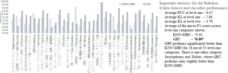
KNN+DBN GBT Important statistics for the Rakuten
Ichiba dataset and classifier performance: - Average PCC at level one – 0.47
- Average KL at level one – 7.88
- Average KL at level two – 3.79
- Average of the micro-F1 scores across level one categories shown:
- KNN+DBN – 73.85
- GBT –76.89*
[image:9.595.76.520.51.193.2]- GBT performs significantly better than KNN+DBN for 28 out of 35 level one categories. There is one other category, Smartphones and Tablets, where GBT performs only slightly better than KNN+DBN.
Figure 11: Comparison of GBTs versus the method from Cevahir and Murakami (2016) on a10% test
set from the Rakuten Ichiba Japanese product listing dataset.
cery” are in one branch, with most other branches
containing less than10listings. In summary, from
both Figs. 9 and 10, we observe that GBTs and CNNs with pre-training perform best even in ex-treme data imbalance. It is possible that GBTs need finer parameter tuning per top-level subtree for datasets resembling AMZ.
5.6 Results on Rakuten Ichiba Dataset In this section, we report our findings on the ef-ficacy of GBTs vis-a-vis another hybrid nearest neighbor and deep learning based method from Cevahir and Murakami (2016). Our decision to employ a tri-level classifier cascade, instead of the bi-level one used for the other datasets, stems from our observations of the KL divergence values (see Section 3 and Table 1) at the first and second level depths of the RAI taxonomy tree. Moving from the first level down to the second decreases the
KL divergence by more than50%. We thus expect
GBTs to perform better due to this reduced imbal-ance. We also cross-validated this assumption on
some popular categories, such as“Clothing”.
From Fig. 11 and the statistics noted therein, we observe that, on average, GBTs outperform the KNN+DBN model from Cevahir and Murakami
(2016) by3percentage points across all top level
categories, which is statistically significant under
a pairedt-test withp <0.0001. As with previous
experiments, only a common best parameter con-figuration has been set for GBTs, without resort-ing to time consumresort-ing cross-validation across all
categories. For the29categories on which GBTs
do better, the mean of the absolute percentage
im-provement is 11.78, with a standard deviation of
5.07. Also, it has been observed that GBTs
sig-nificantly outperform KNN+DBN in28 of those
categories.
The comparison in Fig. 11 is more holistic.
Un-like the top level categorization scores obtained in Figs. 3, 9 and 10, the scores in Fig. 11 have been obtained by categorizing each test example through the entire cascade of hierarchical models for two classifiers. Even with this setting, the per-formance of GBTs is significantly better.
6 Conclusion
Large-scale taxonomy categorization with noisy and imbalanced data is a challenging task. We demonstrate deep learning and gradient tree boost-ing models with operational robustness in real industrial settings for e-commence catalogs with
several millions of items. We summarize our
contributions as follows: 1) We conclude that
GBTs and CNNs can be used as new state-of-the-art baselines for product taxonomy categorization
problems, regardless of the language used; 2)
References
Martn Abadi et al. 2015. Tensorflow: Large-scale machine learning on heterogeneous distributed sys-tems.
Ron Bekkerman and Matan Gavish. 2011. High-precision phrase-based document classification on a modern scale. In Proceedings of the 17th ACM SIGKDD International Conference on Knowledge Discovery and Data Mining, KDD ’11, pages 231– 239, New York, NY, USA. ACM.
Ali Cevahir and Koji Murakami. 2016. Large-scale multi-class and hierarchical product categorization for an e-commerce giant. In Proceedings of COL-ING 2016, the 26th International Conference on Computational Linguistics: Technical Papers, pages 525–535, Osaka, Japan, December. The COLING 2016 Organizing Committee.
Nitesh V. Chawla, Kevin W. Bowyer, Lawrence O. Hall, and W. Philip Kegelmeyer. 2002. Smote: Syn-thetic minority over-sampling technique. J. Artif. Int. Res., 16(1):321–357, June.
Tianqi Chen and Carlos Guestrin. 2016. Xgboost: A scalable tree boosting system. InProceedings of the 22nd ACM SIGKDD International Conference on Knowledge Discovery and Data Mining, San Fran-cisco, CA, USA, August 13-17, 2016, pages 785– 794.
Corinna Cortes and Vladimir Vapnik. 1995. Support-vector networks. Mach. Learn., 20(3):273–297, September.
Thomas M. Cover and Joy A. Thomas. 1991. Ele-ments of Information Theory. Wiley-Interscience, New York, NY, USA.
Pradipto Das, Rohini Srihari, and Yun Fu. 2011. Si-multaneous joint and conditional modeling of docu-ments tagged from two perspectives. InProceedings of the 20th ACM International Conference on In-formation and Knowledge Management, CIKM ’11, pages 1353–1362, New York, NY, USA. ACM. Rong-En Fan, Kai-Wei Chang, Cho-Jui Hsieh,
Xiang-Rui Wang, and Chih-Jen Lin. 2008. Liblinear: A li-brary for large linear classification. J. Mach. Learn. Res., 9:1871–1874, June.
Jerome H. Friedman. 2000. Greedy function approx-imation: A gradient boosting machine. Annals of Statistics, 29:1189–1232.
Venkatesh Ganti, Arnd Christian K¨onig, and Xiao Li. 2010. Precomputing search features for fast and ac-curate query classification. In Proceedings of the Third ACM International Conference on Web Search and Data Mining, WSDM ’10.
Xavier Glorot and Yoshua Bengio. 2010. Understand-ing the difficulty of trainUnderstand-ing deep feedforward neu-ral networks. InIn Proceedings of the International
Conference on Artificial Intelligence and Statistics (AISTATS10). Society for Artificial Intelligence and Statistics.
Trevor Hastie, Robert Tibshirani, and Jerome Fried-man. 2003. The Elements of Statistical Learning: Data Mining, Inference, and Prediction. Springer, August.
Yoon Kim. 2014. Convolutional neural networks for sentence classification. In Proceedings of the 2014 Conference on Empirical Methods in Natu-ral Language Processing (EMNLP), pages 1746– 1751, Doha, Qatar, October. Association for Com-putational Linguistics.
Diederik P. Kingma and Jimmy Ba. 2014. Adam: A method for stochastic optimization. CoRR, abs/1412.6980.
Zornitsa Kozareva. 2015. Everyone likes shopping! multi-class product categorization for e-commerce. In NAACL HLT 2015, The 2015 Conference of the North American Chapter of the Association for Computational Linguistics: Human Language Tech-nologies, Denver, Colorado, USA, May 31 - June 5, 2015, pages 1329–1333.
Y. LeCun and Y. Bengio. 1995. Convolutional net-works for images, speech, and time-series. In M. A. Arbib, editor, The Handbook of Brain Theory and Neural Networks. MIT Press.
Christopher D. Manning, Prabhakar Raghavan, and Hinrich Sch¨utze. 2008. Introduction to Information Retrieval. Cambridge University Press, New York, NY, USA.
Christopher D. Manning, Mihai Surdeanu, John Bauer, Jenny Finkel, Steven J. Bethard, and David Mc-Closky. 2014. The Stanford CoreNLP natural lan-guage processing toolkit. InAssociation for Compu-tational Linguistics (ACL) System Demonstrations, pages 55–60.
Julian McAuley, Rahul Pandey, and Jure Leskovec. 2015. Inferring networks of substitutable and com-plementary products. In Proceedings of the 21th ACM SIGKDD International Conference on Knowl-edge Discovery and Data Mining, KDD ’15, pages 785–794, New York, NY, USA. ACM.
Tomas Mikolov, Ilya Sutskever, Kai Chen, Gregory S. Corrado, and Jeffrey Dean. 2013. Distributed rep-resentations of words and phrases and their com-positionality. In Advances in Neural Information Processing Systems 26: 27th Annual Conference on Neural Information Processing Systems 2013. Pro-ceedings of a meeting held December 5-8, 2013, Lake Tahoe, Nevada, United States., pages 3111– 3119.
Duangmanee (Pew) Putthividhya and Junling Hu. 2011. Bootstrapped named entity recognition for product attribute extraction. In Proceedings of the Conference on Empirical Methods in Natural Lan-guage Processing, EMNLP ’11, pages 1557–1567, Stroudsburg, PA, USA. Association for Computa-tional Linguistics.
Hyuna Pyo, Jung-Woo Ha, and Jeonghee Kim. 2016. Large-scale item categorization in e-commerce us-ing multiple recurrent neural networks. In Proceed-ings of the 22nd ACM SIGKDD International Con-ference on Knowledge Discovery and Data Mining, KDD ’16, New York, NY, USA. ACM.
Dan Shen, Jean David Ruvini, Manas Somaiya, and Neel Sundaresan. 2011. Item categorization in the e-commerce domain. In Proceedings of the 20th ACM International Conference on Information and Knowledge Management, CIKM ’11, pages 1921– 1924, New York, NY, USA. ACM.
Dan Shen, Jean-David Ruvini, Rajyashree Mukherjee, and Neel Sundaresan. 2012a. A study of smoothing algorithms for item categorization on e-commerce sites. Neurocomput., 92:54–60, September.
Dan Shen, Jean-David Ruvini, and Badrul Sarwar. 2012b. Largscale item categorization for e-commerce. In Proceedings of the 21st ACM In-ternational Conference on Information and Knowl-edge Management, CIKM ’12, pages 595–604, New York, NY, USA. ACM.
Chong Sun, Narasimhan Rampalli, Frank Yang, and AnHai Doan. 2014. Chimera: Large-scale classi-fication using machine learning, rules, and crowd-sourcing. Proc. VLDB Endow., 7(13), August. Hsiang-Fu Yu, Chia-Hua Ho, Yu-Chin Juan, and
Chih-Jen Lin. 2013a. LibShortText: A Library for Short-text Classication and Analysis. Technical report, Department of Computer Science, National Taiwan University, Taipei 106, Taiwan.
Hsiang-Fu Yu, Chia hua Ho, Prakash Arunachalam, Manas Somaiya, and Chih jen Lin. 2013b. Product title classification versus text classification. Techni-cal report, UTexas, Austin; NTU; EBay.
Bianca Zadrozny and Charles Elkan. 2002. Trans-forming classifier scores into accurate multiclass probability estimates. InProceedings of the Eighth ACM SIGKDD International Conference on Knowl-edge Discovery and Data Mining, KDD ’02, pages 694–699, New York, NY, USA. ACM.
Tong Zhang. 2004. Solving large scale linear pre-diction problems using stochastic gradient descent algorithms. In ICML 2004: Proceedings of the 21st International Conference on Machine Learn-ing, pages 919–926.
Hui Zou and Trevor Hastie. 2005. Regularization and variable selection via the elastic net. Journal of the Royal Statistical Society, Series B, 67:301–320.
A Supplemental Materials: Model Parameters
In this paper, the baseline classifiers comprise of Na¨ıve Bayes (NB) (Ng and Jordan, 2001) similar to the approach described in Shen et al. (2012a) and Sun et al. (2014), and Logistic Regression
(LogReg) classifiers withL1(Fan et al., 2008) and
Elastic Net regularization. The objective functions
of both GBTs and CNNs involve L2 regularizers
over the set of parameters. Our development set for parameter tuning is generated by randomly
se-lecting 10% of the listings under the “apparel /
clothing” categories. The optimized parameters
obtained from this scaled-down configuration is then extended to all other classifiers to reduce ex-perimentation time.
For parameter tuning, we set a linear
combina-tion of 15%L1 regularization and 85%L2
regu-larization for Elastic Net. For GBTs (Chen and Guestrin, 2016) on both English and Japanese data, we limit each decision tree growth to a
max-imum depth of 500 and the number of boosting
rounds is set to 50. Additionally, for leaf node
weights, we use L2 regularization with a
regu-larization constant of 0.5. For GBTs on English
data, the initial learning rate is0.2. For GBTs on
Japanese data, the initial learning rate is assigned
a value of0.05.
For CNNs, we use context window widths of
sizes1,3,4,5for four convolution filters, a batch
size of 1024 and an embedding dimension of
300. The parameters for the embeddings are non-static. The convolutional filters are initial-ized with Xavier initialization (Glorot and Ben-gio, 2010). We use mini-batch stochastic gradi-ent descgradi-ent with Adam optimizer (Kingma and Ba, 2014) to perform parameter optimization.