Very Deep Convolutional Networks
for Text Classification
Alexis Conneau
Facebook AI Research
Holger Schwenk
Facebook AI Research
Yann Le Cun
Facebook AI Research
Lo¨ıc Barrault
LIUM, University of Le Mans, France
Abstract
The dominant approach for many NLP tasks are recurrent neural networks, in par-ticular LSTMs, and convolutional neural networks. However, these architectures are rather shallow in comparison to the deep convolutional networks which have pushed the state-of-the-art in computer vi-sion. We present a new architecture (VD-CNN) for text processing which operates directly at the character level and uses only small convolutions and pooling oations. We are able to show that the per-formance of this model increases with the depth: using up to 29 convolutional layers, we report improvements over the state-of-the-art on several public text classification tasks. To the best of our knowledge, this is the first time that very deep convolutional nets have been applied to text processing.
1 Introduction
The goal of natural language processing (NLP) is to process text with computers in order to analyze it, to extract information and eventually to rep-resent the same information differently. We may want to associate categories to parts of the text (e.g. POS tagging or sentiment analysis), struc-ture text differently (e.g. parsing), or convert it to some other form which preserves all or part of the content (e.g. machine translation, summariza-tion). The level of granularity of this processing can range from individual characters to subword units (Sennrich et al., 2016) or words up to whole sentences or even paragraphs.
After a couple of pioneer works (Bengio et al. (2001), Collobert and Weston (2008), Collobert et al. (2011) among others), the use of neural net-works for NLP applications is attracting huge
in-terest in the research community and they are sys-tematically applied to all NLP tasks. However, while the use of (deep) neural networks in NLP has shown very good results for many tasks, it seems that they have not yet reached the level to outperform the state-of-the-art by a large margin, as it was observed in computer vision and speech recognition.
Convolutional neural networks, in short Con-vNets, are very successful in computer vision. In early approaches to computer vision, handcrafted features were used, for instance “scale-invariant feature transform (SIFT)”(Lowe, 2004), followed by some classifier. The fundamental idea of Con-vNets(LeCun et al., 1998) is to consider feature extraction and classification as one jointly trained task. This idea has been improved over the years, in particular by using many layers of convolutions and pooling to sequentially extract a hierarchical representation(Zeiler and Fergus, 2014) of the in-put. The best networks are using more than 150 layers as in (He et al., 2016a; He et al., 2016b).
Many NLP approaches consider words as ba-sic units. An important step was the introduction of continuous representations of words(Bengio et al., 2003). Theseword embeddings are now the state-of-the-art in NLP. However, it is less clear how we should best represent a sequence of words, e.g. a whole sentence, which has complicated syn-tactic and semantic relations. In general, in the same sentence, we may be faced with local and long-range dependencies. Currently, the main-stream approach is to consider a sentence as a se-quence of tokens (characters or words) and to pro-cess them with a recurrent neural network (RNN). Tokens are usually processed in sequential order, from left to right, and the RNN is expected to
“memorize” the whole sequence in its internal states. The most popular and successful RNN vari-ant are certainly LSTMs(Hochreiter and
Dataset Label Sample
Yelp P. +1 Been going to Dr. Goldberg for over 10 years. I think I was one of his 1st patients when he started at MHMG. Hes been great over the years and is really all about the big picture. [...]
Amz P. 3(/5) I love this show, however, there are 14 episodes in the first season and this DVD only shows the first eight. [...]. I hope the BBC will release another DVD that contains all the episodes, but for now this one is still somewhat enjoyable. Sogou ”Sports” ju4 xi1n hua2 she4 5 yue4 3 ri4 , be3i ji1ng 2008 a4o yu4n hui4 huo3 ju4 jie1
li4 ji1ng guo4 shi4 jie4 wu3 da4 zho1u 21 ge4 che2ng shi4 Yah. A. ”Computer,
Internet” ”What should I look for when buying a laptop? What is the best brand andwhat’s reliable?”,”Weight and dimensions are important if you’re planning to travel with the laptop. Get something with at least 512 mb of RAM. [..] is a good brand, and has an easy to use site where you can build a custom laptop.”
Table 1: Examples of text samples and their labels.
huber, 1997) – there are many works which have shown the ability of LSTMs to model long-range dependencies in NLP applications, e.g. (Sunder-meyer et al., 2012; Sutskever et al., 2014) to name just a few. However, we argue that LSTMs are generic learning machines for sequence process-ing which are lackprocess-ing task-specific structure.
We propose the following analogy. It is well known that a fully connected one hidden layer neural network can in principle learn any real-valued function, but much better results can be obtained with a deep problem-specific architec-ture which develops hierarchical representations. By these means, the search space is heavily con-strained and efficient solutions can be learned with gradient descent. ConvNets are namely adapted for computer vision because of the compositional structure of an image. Texts have similar proper-ties : characters combine to form n-grams, stems, words, phrase, sentences etc.
We believe that a challenge in NLP is to develop deep architectures which are able to learn hierar-chical representations of whole sentences, jointly with the task. In this paper, we propose to use deep architectures of many convolutional layers to ap-proach this goal, using up to 29 layers. The design of our architecture is inspired by recent progress in computer vision, in particular (Simonyan and Zisserman, 2015; He et al., 2016a).
This paper is structured as follows. There have been previous attempts to use ConvNets for text processing. We summarize the previous works in the next section and discuss the relations and dif-ferences. Our architecture is described in detail in section 3. We have evaluated our approach on
several sentence classification tasks, initially pro-posed by (Zhang et al., 2015). These tasks and our experimental results are detailed in section 4. The proposed deep convolutional network shows significantly better results than previous ConvNets approach. The paper concludes with a discus-sion of future research directions for very deep ap-proach in NLP.
2 Related work
There is a large body of research on sentiment analysis, or more generally on sentence classifica-tion tasks. Initial approaches followed the clas-sical two stage scheme of extraction of (hand-crafted) features, followed by a classification stage. Typical features include bag-of-words or n-grams, and their TF-IDF. These techniques have been compared with ConvNets by (Zhang et al., 2015; Zhang and LeCun, 2015). We use the same corpora for our experiments. More recently, words or characters, have been projected into a low-dimensional space, and these embeddings are combined to obtain a fixed size representation of the input sentence, which then serves as input for the classifier. The simplest combination is the element-wise mean. This usually performs badly since all notion of token order is disregarded.
net-work (RNN) could be considered as a special case of a recursive NN: the combination is performed sequentially, usually from left to right. The last state of the RNN is used as fixed-sized representa-tion of the sentence, or eventually a combinarepresenta-tion of all the hidden states.
First works using convolutional neural networks for NLP appeared in (Collobert and Weston, 2008; Collobert et al., 2011). They have been subse-quently applied to sentence classification (Kim, 2014; Kalchbrenner et al., 2014; Zhang et al., 2015). We will discuss these techniques in more detail below. If not otherwise stated, all ap-proaches operate on words which are projected into a high-dimensional space.
A rather shallow neural net was proposed in (Kim, 2014): one convolutional layer (using multiple widths and filters) followed by a max pooling layer over time. The final classifier uses one fully connected layer with drop-out. Results are reported on six data sets, in particular Stanford Sentiment Treebank (SST). A similar system was proposed in (Kalchbrenner et al., 2014), but us-ing five convolutional layers. An important differ-ence is also the introduction of multipletemporal k-max poolinglayers. This allows to detect thek most important features in a sentence, independent of their specific position, preserving their relative order. The value of k depends on the length of the sentence and the position of this layer in the network. (Zhang et al., 2015) were the first to per-form sentiment analysis entirely at the character level. Their systems use up to six convolutional layers, followed by three fully connected classifi-cation layers. Convolutional kernels of size 3 and 7 are used, as well as simple max-pooling layers. Another interesting aspect of this paper is the in-troduction of several large-scale data sets for text classification. We use the same experimental set-ting (see section 4.1). The use of character level information was also proposed by (Dos Santos and Gatti, 2014): all the character embeddings of one word are combined by a max operation and they are then jointly used with the word embedding in-formation in a shallow architecture. In parallel to our work, (Yang et al., 2016) proposed a based hi-erarchical attention network for document classi-fication that perform an attention first on the sen-tences in the document, and on the words in the sentence. Their architecture performs very well on datasets whose samples contain multiple
sen-tences.
In the computer vision community, the com-bination of recurrent and convolutional networks in one architecture has also been investigated, with the goal to “get the best of both worlds”, e.g. (Pinheiro and Collobert, 2014). The same idea was recently applied to sentence classifica-tion (Xiao and Cho, 2016). A convoluclassifica-tional net-work with up to five layers is used to learn high-level features which serve as input for an LSTM. The initial motivation of the authors was to ob-tain the same performance as (Zhang et al., 2015) with networks which have significantly fewer pa-rameters. They report results very close to those of (Zhang et al., 2015) or even outperform Con-vNets for some data sets.
In summary, we are not aware of any work that uses VGG-like or ResNet-like architecture to go deeper than than six convolutional layers (Zhang et al., 2015) for sentence classification. Deeper networks were not tried or they were re-ported to not improve performance. This is in sharp contrast to the current trend in computer vi-sion where significant improvements have been re-ported using much deeper networks(Krizhevsky et al., 2012), namely 19 layers (Simonyan and Zis-serman, 2015), or even up to 152 layers (He et al., 2016a). In the remainder of this paper, we describe our very deep convolutional architecture and re-port results on the same corpora than (Zhang et al., 2015). We were able to show that performance improves with increased depth, using up to 29 con-volutional layers.
3 VDCNN Architecture
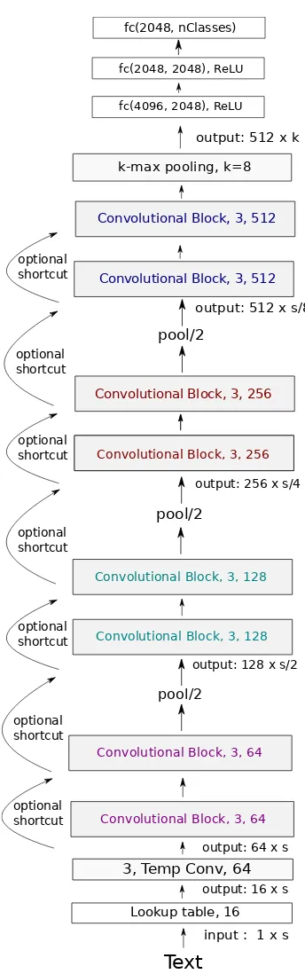
The overall architecture of our network is shown in Figure 1. Our model begins with a look-up ta-ble that generates a 2D tensor of size(f0, s) that contain the embeddings of thes characters. sis fixed to 1024, and f0 can be seen as the ”RGB” dimension of the input text.
tempo-Text
Lookup table, 16
Convolutional Block, 3, 64 Convolutional Block, 3, 128 Convolutional Block, 3, 256
Convolutional Block, 3, 512
3, Temp Conv, 64
k-max pooling, k=8
input : 1 x s output: 512 x k
fc(4096, 2048), ReLU
output: 16 x s output: 64 x s
fc(2048, 2048), ReLU
fc(2048, nClasses)
Convolutional Block, 3, 128
output: 128 x s/2 Convolutional Block, 3, 256 Convolutional Block, 3, 256
output: 256 x s/4
Convolutional Block, 3, 512
output: 512 x s/8
pool/2
Convolutional Block, 3, 64
pool/2 pool/2
optional shortcut optional shortcut optional shortcut optional shortcut
optional shortcut
optional shortcut
[image:4.595.93.265.123.672.2]optional shortcut
Figure 1: VDCNN architecture.
ral resolution each time by 2), resulting in 3 levels of 128, 256 and 512 feature maps (see Figure 1). The output of these convolutional blocks is a ten-sor of size512×sd, where sd = 2sp with p = 3 the number of down-sampling operations. At this level of the convolutional network, the resulting tensor can be seen as a high-level representation of the input text. Since we deal with padded in-put text of fixed size, sd is constant. However,
in the case of variable size input, the convolu-tional encoder provides a representation of the in-put text that depends on its initial lengths. Repre-sentations of a text as a set of vectors of variable size can be valuable namely for neural machine translation, in particular when combined with an attention model. In Figure 1, temporal convolu-tions with kernel size 3 and X feature maps are denoted ”3, Temp Conv, X”, fully connected layers which are linear projections (matrix of size I ×O) are denoted ”fc(I, O)” and ”3-max pooling, stride 2” means temporal max-pooling with kernel size 3 and stride 2.
Most of the previous applications of ConvNets to NLP use an architecture which is rather shal-low (up to 6 convolutional layers) and combines convolutions of different sizes, e.g. spanning 3, 5 and 7 tokens. This was motivated by the fact that convolutions extract n-gram features over tokens and that different n-gram lengths are needed to model short- and long-span relations. In this work, we propose to create instead an architecture which uses many layers of small convolutions (size 3). Stacking 4 layers of such convolutions results in a span of 9 tokens, but the network can learn by it-self how to best combine these different“3-gram features” in a deep hierarchical manner. Our ar-chitecture can be in fact seen as a temporal adap-tation of the VGG network (Simonyan and Zisser-man, 2015). We have also investigated the same kind of“ResNet shortcut”connections as in (He et al., 2016a), namely identity and1×1 convolu-tions (see Figure 1).
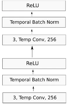
Figure 2: Convolutional block.
hidden units and softmax outputs. The number of output neurons depends on the classification task, the number of hidden units is set to 2048, andk to 8 in all experiments. We do not use drop-out with the fully connected layers, but only temporal batch normalization after convolutional layers to regularize our network.
Convolutional Block
Each convolutional block (see Figure 2) is a se-quence of two convolutional layers, each one followed by a temporal BatchNorm (Ioffe and Szegedy, 2015) layer and an ReLU activation. The kernel size of all the temporal convolutions is 3, with padding such that the temporal resolution is preserved (or halved in the case of the convolu-tional pooling with stride 2, see below). Steadily increasing the depth of the network by adding more convolutional layers is feasible thanks to the limited number of parameters of very small con-volutional filters in all layers. Different depths of the overall architecture are obtained by vary-ing the number of convolutional blocks in between the pooling layers (see table 2). Temporal batch normalization applies the same kind of regulariza-tion as batch normalizaregulariza-tion except that the activa-tions in a mini-batch are jointly normalized over temporal (instead of spatial) locations. So, for a mini-batch of sizemand feature maps of tempo-ral sizes, the sum and the standard deviations re-lated to the BatchNorm algorithm are taken over
|B|=m·sterms.
We explore three types of down-sampling be-tween blocksKiandKi+1(Figure 1) :
(i) The first convolutional layer of Ki+1 has stride 2 (ResNet-like).
Depth: 9 17 29 49
conv block 512 2 4 4 6
conv block 256 2 4 4 10
conv block 128 2 4 10 16
conv block 64 2 4 10 16
First conv. layer 1 1 1 1
#params [in M] 2.2 4.3 4.6 7.8
Table 2: Number of conv. layers per depth. (ii) Ki is followed by a k-max pooling layer
wherekis such that the resolution is halved (Kalchbrenner et al., 2014).
(iii) Ki is followed by max-pooling with kernel
size 3 and stride 2 (VGG-like).
All these types of pooling reduce the temporal res-olution by a factor 2. At the final convres-olutional layer, the resolution is thussd.
In this work, we have explored four depths for our networks: 9, 17, 29 and 49, which we de-fine as being the number of convolutional lay-ers. The depth of a network is obtained by sum-ming the number of blocks with 64, 128, 256 and 512 filters, with each block containing two con-volutional layers. In Figure 1, the network has 2 blocks of each type, resulting in a depth of
2×(2 + 2 + 2 + 2) = 16. Adding the very first convolutional layer, this sums to a depth of 17 con-volutional layers. The depth can thus be increased or decreased by adding or removing convolutional blocks with a certain number of filters. The best configurations we observed for depths 9, 17, 29 and 49 are described in Table 2. We also give the number of parameters of all convolutional layers.
4 Experimental evaluation 4.1 Tasks and data
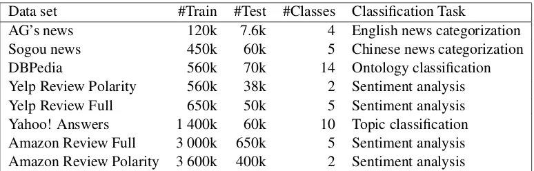
[image:5.595.321.511.62.158.2]Data set #Train #Test #Classes Classification Task
AG’s news 120k 7.6k 4 English news categorization
Sogou news 450k 60k 5 Chinese news categorization
DBPedia 560k 70k 14 Ontology classification
Yelp Review Polarity 560k 38k 2 Sentiment analysis
Yelp Review Full 650k 50k 5 Sentiment analysis
Yahoo! Answers 1 400k 60k 10 Topic classification
Amazon Review Full 3 000k 650k 5 Sentiment analysis
[image:6.595.106.493.61.185.2]Amazon Review Polarity 3 600k 400k 2 Sentiment analysis
Table 3: Large-scale text classification data sets used in our experiments. See (Zhang et al., 2015) for a detailed description.
and 14. This is considerably lower than in com-puter vision (e.g. 1 000 classes for ImageNet). This has the consequence that each example in-duces less gradient information which may make it harder to train large architectures. It should be also noted that some of the tasks are very ambigu-ous, in particular sentiment analysis for which it is difficult to clearly associate fine grained labels. There are equal numbers of examples in each class for both training and test sets. The reader is re-ferred to (Zhang et al., 2015) for more details on the construction of the data sets. Table 4 summa-rizes the best published results on these corpora we are aware of. We do not use “Thesaurus data augmentation” or any other preprocessing, except lower-casing. Nevertheless, we still outperform the best convolutional neural networks of (Zhang et al., 2015) for all data sets. The main goal of our work is to show that it is possible and beneficial to train very deep convolutional networks as text encoders. Data augmentation may improve our re-sults even further. We will investigate this in future research.
4.2 Common model settings
The following settings have been used in all our experiments. They were found to be best in initial experiments. Following (Zhang et al., 2015), all processing is done at the char-acter level which is the atomic representation of a sentence, same as pixels for images. The dictionary consists of the following characters ”abcdefghijklmnopqrstuvwxyz0123456 789-,;.!?:’"/| #$%ˆ&*˜‘+=<>()[]{}” plus a special padding, space and unknown token which add up to a total of 69 tokens. The input text is padded to a fixed size of 1014, larger text are truncated. The character embedding is
of size 16. Training is performed with SGD, using a mini-batch of size 128, an initial learning rate of 0.01 and momentum of 0.9. We follow the same training procedure as in (Zhang et al., 2015). We initialize our convolutional layers following (He et al., 2015). One epoch took from 24 minutes to 2h45 for depth 9, and from 50 minutes to 7h (on the largest datasets) for depth 29. It took between 10 to 15 epoches to converge. The implementation is done using Torch 7. All experiments are performed on a single NVidia K40 GPU. Unlike previous research on the use of ConvNets for text processing, we use temporal batch norm without dropout.
4.3 Experimental results
In this section, we evaluate several configurations of our model, namely three different depths and three different pooling types (see Section 3). Our main contribution is a thorough evaluation of net-works of increasing depth using an architecture with small temporal convolution filters with dif-ferent types of pooling, which shows that a signif-icant improvement on the state-of-the-art configu-rations can be achieved on text classification tasks by pushing the depth to 29 convolutional layers.
Corpus: AG Sogou DBP. Yelp P. Yelp F. Yah. A. Amz. F. Amz. P.
Method n-TFIDF n-TFIDF n-TFIDF ngrams Conv Conv+RNN Conv Conv
Author [Zhang] [Zhang] [Zhang] [Zhang] [Zhang] [Xiao] [Zhang] [Zhang]
Error 7.64 2.81 1.31 4.36 37.95∗ 28.26 40.43∗ 4.93∗
[Yang] - - - 24.2 36.4
-Table 4: Best published results from previous work. Zhang et al. (2015) best results use a Thesaurus data augmentation technique (marked with an ∗). Yang et al. (2016)’s hierarchical methods is particularly adapted to datasets whose samples contain multiple sentences.
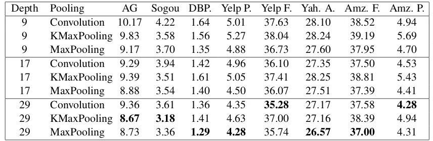
Depth Pooling AG Sogou DBP. Yelp P. Yelp F. Yah. A. Amz. F. Amz. P.
9 Convolution 10.17 4.22 1.64 5.01 37.63 28.10 38.52 4.94
9 KMaxPooling 9.83 3.58 1.56 5.27 38.04 28.24 39.19 5.69
9 MaxPooling 9.17 3.70 1.35 4.88 36.73 27.60 37.95 4.70
17 Convolution 9.29 3.94 1.42 4.96 36.10 27.35 37.50 4.53
17 KMaxPooling 9.39 3.51 1.61 5.05 37.41 28.25 38.81 5.43
17 MaxPooling 8.88 3.54 1.40 4.50 36.07 27.51 37.39 4.41
29 Convolution 9.36 3.61 1.36 4.35 35.28 27.17 37.58 4.28
29 KMaxPooling 8.67 3.18 1.41 4.63 37.00 27.16 38.39 4.94
29 MaxPooling 8.73 3.36 1.29 4.28 35.74 26.57 37.00 4.31
Table 5: Testing error of our models on the 8 data sets. No data preprocessing or augmentation is used. be observed on the largest data set Amazon Full
which has more than 3 Million training samples. We also observe that for a small depth, temporal max-pooling works best on all data sets.
Depth improves performance. As we increase the network depth to 17 and 29, the test errors decrease on all data sets, for all types of pooling (with 2 exceptions for 48 comparisons). Going from depth 9 to 17 and 29 for Amazon Full re-duces the error rate by 1% absolute. Since the test is composed of 650K samples, 6.5K more test samples have been classified correctly. These improvements, especially on large data sets, are significant and show that increasing the depth is useful for text processing. Overall, compared to previous state-of-the-art, our best architecture with depth 29 and max-pooling has a test error of 37.0 compared to 40.43%. This represents a gain of 3.43% absolute accuracy. The significant im-provements which we obtain on all data sets com-pared to Zhang’s convolutional models do not in-clude any data augmentation technique.
Max-pooling performs better than other pool-ing types. In terms of pooling, we can also see that max-pooling performs best overall, very close to convolutions with stride 2, but both are signifi-cantly superior tok-max pooling.
Both pooling mechanisms perform a max oper-ation which is local and limited to three
consec-utive tokens, while k-max polling considers the whole sentence at once. According to our exper-iments, it seems to hurt performance to perform this type of max operation at intermediate layers (with the exception of the smallest data sets).
[image:7.595.84.512.185.325.2]mecha-nism that apply very well to documents (with mul-tiple sentences).
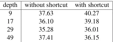
Going even deeper degrades accuracy. Short-cut connections help reduce the degradation.
As described in (He et al., 2016a), the gain in accu-racy due to the the increase of the depth is limited when using standard ConvNets. When the depth increases too much, the accuracy of the model gets saturated and starts degrading rapidly. This degra-dationproblem was attributed to the fact that very deep models are harder to optimize. The gradi-ents which are backpropagated through the very deep networks vanish and SGD with momentum is not able to converge to a correct minimum of the loss function. To overcome this degradation of the model, theResNet modelintroduced short-cut connections between convolutional blocks that allow the gradients to flow more easily in the net-work (He et al., 2016a).
We evaluate the impact of shortcut connections by increasing the number of convolutions to 49 layers. We present an adaptation of the ResNet model to the case of temporal convolutions for text (see Figure 1). Table 6 shows the evolution of the test errors on the Yelp Review Full data set with or without shortcut connections. When looking at the column “without shortcut”, we observe the same degradation problem as in the original ResNet ar-ticle: when going from 29 to 49 layers, the test error rate increases from 35.28 to 37.41 (while the training error goes up from 29.57 to 35.54). When using shortcut connections, we observe improved results when the network has 49 layers: both the training and test errors go down and the network is less prone to underfitting than it was without short-cut connections.
While shortcut connections give better results when the network is very deep (49 layers), we were not able to reach state-of-the-art results with them. We plan to further explore adaptations of residual networks to temporal convolutions as we think this a milestone for going deeper in NLP. Residual units (He et al., 2016a) better adapted to the text processing task may help for training even deeper models for text processing, and is left for future research.
Exploring these models on text classification tasks with more classes sounds promising.
Note that one of the most important difference between the classification tasks discussed in this
depth without shortcut with shortcut
9 37.63 40.27
17 36.10 39.18
29 35.28 36.01
[image:8.595.323.511.61.131.2]49 37.41 36.15
Table 6: Test error on the Yelp Full data set for all depths, with or without residual connections.
work and ImageNet is that the latter deals with 1000 classes and thus much more information is back-propagated to the network through the gra-dients. Exploring the impact of the depth of tem-poral convolutional models on categorization tasks with hundreds or thousands of classes would be an interesting challenge and is left for future research.
5 Conclusion
We have presented a new architecture for NLP which follows two design principles: 1) operate at the lowest atomic representation of text, i.e. char-acters, and 2) use a deep stack of local operations, i.e. convolutions and max-pooling of size 3, to learn a high-level hierarchical representation of a sentence. This architecture has been evaluated on eight freely available large-scale data sets and we were able to show that increasing the depth up to 29 convolutional layers steadily improves perfor-mance. Our models are much deeper than pre-viously published convolutional neural networks and they outperform those approaches on all data sets. To the best of our knowledge, this is the first time that the “benefit of depths” was shown for convolutional neural networks in NLP.
Eventhough text follows human-defined rules and images can be seen as raw signals of our en-vironment, images and small texts have similar properties. Texts are also compositional for many languages. Characters combine to form n-grams, stems, words, phrase, sentences etc. These simi-lar properties make the comparison between com-puter vision and natural language processing very profitable and we believe future research should invest into making text processing models deeper. Our work is a first attempt towards this goal.
References
Yoshua Bengio, Rejean Ducharme, and Pascal Vin-cent. 2001. A neural probabilistic language model. In NIPS, volume 13, pages 932–938, Vancouver, British Columbia, Canada.
Yoshua Bengio, R´ejean Ducharme, Pascal Vincent, and Christian Jauvin. 2003. A neural probabilistic lan-guage model. Journal of machine learning research, 3(Feb):1137–1155.
Ronan Collobert and Jason Weston. 2008. A unified architecture for natural language processing: deep neural networks with multitask learning. InICML, pages 160–167, Helsinki, Finland.
Ronan Collobert, Jason Weston Lon Bottou, M. Karlen, K. Kavukcuoglu, and P. Kuksa. 2011. Natural language processing (almost) from scratch. JMLR, pages 2493–2537.
C´ıcero Nogueira Dos Santos and Maira Gatti. 2014. Deep convolutional neural networks for sentiment analysis of short texts. In COLING, pages 69–78, Dublin, Ireland.
Kaiming He, Xiangyu Zhang, Shaoqing Ren, and Jian Sun. 2015. Delving deep into rectifiers: Surpass-ing human-level performance on imagenet classifi-cation. In Proceedings of the IEEE international conference on computer vision, pages 1026–1034, Santiago, Chile.
Kaiming He, Xiangyu Zhang, Shaoqing Ren, and Jian Sun. 2016a. Deep residual learning for image recognition. InProceedings of the IEEE Conference on Computer Vision and Pattern Recognition, pages 770–778, Las Vegas, Nevada, USA.
Kaiming He, Xiangyu Zhang, Shaoqing Ren, and Jian Sun. 2016b. Identity mappings in deep residual networks. In European Conference on Computer Vision, pages 630–645, Amsterdam, Netherlands. Springer.
Sepp Hochreiter and J¨urgen Schmidhuber. 1997. Long short-term memory. Neural computation, 9(8):1735–1780.
Sergey Ioffe and Christian Szegedy. 2015. Batch nor-malization: Accelerating deep network training by reducing internal covariate shift. In ICML, pages 448–456, Lille, France.
Nal Kalchbrenner, Edward Grefenstette, and Phil Blun-som. 2014. A convolutional neural network for modelling sentences. In Proceedings of the 52nd Annual Meeting of the Association for Computa-tional Linguistics, pages 655–665, Baltimore, Mary-land, USA.
Yoon Kim. 2014. Convolutional neural networks for sentence classification. In Proceedings of the 2014 Conference on Empirical Methods in Natural Language Processing (EMNLP), pages 1746–1751,
Doha, Qatar. Association for Computational Lin-guistics.
Alex Krizhevsky, Ilya Sutskever, and Geoffrey E Hin-ton. 2012. Imagenet classification with deep con-volutional neural networks. In Advances in neural information processing systems, pages 1097–1105, Lake Tahoe, California, USA.
Yann LeCun, L´eon Bottou, Yoshua Bengio, and Patrick Haffner. 1998. Gradient-based learning applied to document recognition. Proceedings of the IEEE, 86(11):2278–2324.
David G Lowe. 2004. Distinctive image features from scale-invariant keypoints. International journal of computer vision, 60(2):91–110.
Pedro HO Pinheiro and Ronan Collobert. 2014. Re-current convolutional neural networks for scene la-beling. InICML, pages 82–90, Beijing, China. Rico Sennrich, Barry Haddow, and Alexandra Birch.
2016. Neural machine translation of rare words with subword units. pages 1715–1725.
Karen Simonyan and Andrew Zisserman. 2015. Very deep convolutional networks for large-scale image recognition. InICLR, San Diego, California, USA.
Richard Socher, Jeffrey Pennington, Eric H Huang, Andrew Y Ng, and Christopher D Manning. 2011. Semi-supervised recursive autoencoders for predict-ing sentiment distributions. In Proceedings of the conference on empirical methods in natural lan-guage processing, pages 151–161, Edinburgh, UK. Association for Computational Linguistics.
Martin Sundermeyer, Ralf Schl¨uter, and Hermann Ney. 2012. Lstm neural networks for language model-ing. InInterspeech, pages 194–197, Portland, Ore-gon, USA.
Ilya Sutskever, Oriol Vinyals, and Quoc V. Le. 2014. Sequence to sequence learning with neural net-works. In NIPS, pages 3104–3112, Montreal, Canada.
Yijun Xiao and Kyunghyun Cho. 2016. Efficient character-level document classification by combin-ing convolution and recurrent layers.
Zichao Yang, Diyi Yang, Chris Dyer, Xiaodong He, Alex Smola, and Eduard Hovy. 2016. Hierarchi-cal attention networks for document classification. In Proceedings of NAACL-HLT, pages 1480–1489, San Diego, California, USA.
Matthew D Zeiler and Rob Fergus. 2014. Visualizing and understanding convolutional networks. In Eu-ropean conference on computer vision, pages 818– 833, Zurich, Switzerland. Springer.