Proceedings of the 2019 Conference on Empirical Methods in Natural Language Processing
3597
Single Training Dimension Selection for Word Embedding with PCA
Yu Wang Apple [email protected]
Abstract
In this paper, we present a fast and reliable method based on PCA to select the number of dimensions for word embeddings. First, we train one embedding with a generous upper bound (e.g. 1,000) of dimensions. Then we transform the embeddings using PCA and in-crementally remove the lesser dimensions one at a time while recording the embeddings’ per-formance on language tasks. Lastly, we se-lect the number of dimensions while balancing model size and accuracy. Experiments using various datasets and language tasks demon-strate that we are able to train 10 times fewer sets of embeddings while retaining optimal performance. Researchers interested in train-ing the best-performtrain-ing embeddtrain-ings for down-stream tasks, such as sentiment analysis, ques-tion answering and hypernym extracques-tion, as well as those interested in embedding com-pression should find the method helpful.
1 Introduction
Word embeddings constitute an integral part of the implementation of numerous NLP tasks ranging from sentiment classification (Lin et al., 2015), nationality classification (Ye et al.,2017), classi-fication of behavior on Twitter (Wang et al.,2017), to measuring document similarity (Kusner et al.,
2015). The strength of word embeddings stems from their embedding words into low dimensional continuous vector space (Mnih and Kavukcuoglu,
2013;Pennington et al., 2014;Tang et al., 2015;
Raunak,2017).
Various algorithms have been proposed for learning words’ vector space representations, in-cluding most notably Mikolov et al. (2013b), Pen-nington et al. (2014), and Nickel and Kiela (2017). However, the exact definition of ‘low’ dimension-ality is rarely explored. As pointed out by Yin and Shen (2018), the most frequently used dimension-ality is 300, largely due to the fact that the early
influential papers (Mikolov et al., 2013b;
Pen-nington et al.,2014) used 300. Other often used
dimensionalities include 200 (Tang et al., 2015;
Ling et al., 2016; Nickel and Kiela, 2017) and
500 (Tang and Liu,2009;Perozzi et al.,2014). The impact of vector dimension on embed-dings’ performance is well known (Lai et al.,
2016). With too few dimensions, the model will underfit; with too many dimensions the model will overfit. Both undercut the embeddings’ perfor-mance (Yin and Shen,2018). What is also known is that the size of the embeddings will grow lin-early with the vector dimension (Ling et al.,2016;
Raunak, 2017). What is less known is how to
identify the optimal vector dimension given any dataset. The method we propose here helps fill this gap.
100 200 300 400 500
# Dimension
30 32 34 36 38 40
Accuracy
Word Analogy
0 100 200 300 400 500
# Dimension
0.0 0.5 1.0 1.5 2.0 2.5 3.0 3.5
# Parameters
[image:1.595.309.522.466.577.2]1e7 Embedding Size
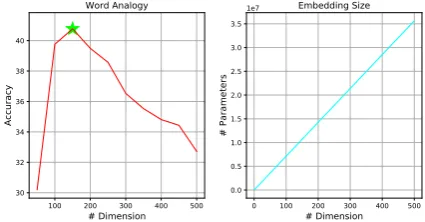
Figure 1: Left: Accuracy for the word analogy task as a function of vector dimension (dimension incremental is 50). Right: The number of embedding parameters as a function of vector dimension. Results are gener-ated using the Text8 dataset with a vocabulary size of 71,291.
We offer a fast and reliable PCA-based method that (1) only needs to train the embeddings once and (2) is able to select vector dimension with competitive performance.1 First, we train one em-bedding with a generous upper bound (e.g. 1,000)
1As such, the selected dimension is a Pareto-optimal
of dimensions. Then we transform the embed-dings using PCA and incrementally remove the lesser dimensions one at a time while recording the embeddings’ performance on language tasks. Lastly we calculate the best dimensionality and re-turn the corresponding embeddings.
Experiments using various datasets and lan-guage tasks reveal three key observations:
• The optimal dimensionality calculated on the basis of PCA agrees with that by grid search.
• The resulting embedding is competitive against the one selected by grid search.
• Different upper-bound dimensionalities (e.g. 500, 1000) point to the same optimal dimen-sionality.
Researchers interested in downstream tasks, such as sentiment analysis (Lin et al.,2015), question answering (Devlin et al.,2018) and hypernym ex-traction (Chen et al.,2018), as well as those inter-ested in embedding compression should find the method helpful.
2 Related Work
Our work draws inspiration from Yin and Shen (2018). The authors build on the Latent Se-mantics Analysis (LSA) approach and slidekfrom a lower bound (e.g. 10) to a generous upper bound (e.g. 1,000) in E = U1:kD1:k,1:kα , where U and D come from the singular-value decomposition of the signal matrix andα is a hyperparameter to be tuned. For eachk, the authors generate one corre-sponding embedding and compare it with the sim-ulated oracle embedding. The k that yields the smallest loss is selected. In a similar vein, our work bypasses the problem of training multiple embeddings, often necessitated by grid search, by sliding over all the k values of PCA. Compared with Yin and Shen (2018), our method is easier to implement, as we do not rely on, e.g, Monte Carlo simulations of the oracle embeddings.
At a deeper level, our work is also connected to Yin and Shen (2018) in terms of the trade-off between bias and variance. Yin and Shen (2018) propose pairwise inner product (PIP) loss to mea-sure the quality of an embedding. They decom-pose the PIP loss into a bias term and a variance term, where reducing the dimension increases the bias term but reduces the variance. They show
that the bias-variance trade-off reflects the signal-to-noise ratio in dimension selection. While there is no exact 1-1 mapping from their theorem to our work, we do have analogous discussion in Section 3. The PCA step in our algorithm enables us to identify and drop dimensions that (1) contribute less to the explained variance in the embedding and yet (2) contribute equally to cosine similarity. In essence, our PCA step is removing dimensions with low signal-to-noise ratios.
Our work also draws strength from the liter-ature on post-processing embeddings. Mu and Viswanath (2018) demonstrate that removing the top dominating directions in the PCA-transformed embeddings helps improve the embeddings’ per-formance in word analogy and similarity tasks. Building on that, Raunak (2017) shows that by performing another iteration of PCA and dropping the bottom directions, one can further improve a model’s performance as well as reduce its size. Both works focus on improving pre-trained em-beddings’s performance in terms of accuracy and size. By contrast, our algorithm selects the opti-mal dimensionality before the actual training.
In addition, our work is related to a few re-cent studies on model compression (Faruqui et al.,
2015; Ling et al., 2016; Shu and Nakayama,
2018). In particular, Ling et al. (2016) seek to drop the least significant digits to reduce the em-beddings’ size. By comparison, our method re-moves the least significant dimensions (in terms of explained variance (Bishop,2006)). It should be noted that the two methods complement each other, as one focuses on dimension selection whereas the other on limited precision represen-tation.
3 Algorithm
In this section, we formally describe how to se-lect a competitive dimensionality by training one embedding. We state the proposed algorithm in Algorithm 1.
First, we note that the PCA transformation (when retaining all the N dimensions) does not affect embeddings’ performance on word similar-ity tasks. Any potential performance gain should come from dropping the lesser dimensions. By “lesser dimensions,” we mean the dimensions that contribute little to the explanation of variance (Bishop,2006).
Algorithm 1Select the Optimal Dimensionality using PCA
Set dimension upper bound N; select language task from{word analogy, similarity}
Train embeddingEwith N dimensions
TransformEusing PCA:(u1, u2, ..., uN; ˜E)←PCA(E), whereu1, u2, .., uN are the new basis vectors,E˜represents the transformed coefficients
fori=N to 2do
E=E-E˜:,i·ui, whereE˜:,irepresents theith column ofE˜ and each scalar inE˜:,iscales vectorui EvaluateEon the selected language task, record (i, metric)
end for
Return the selected dimension: [argmax i
f(i, metric)]-1, wheref is a score function that balances
performance and model size and i is between 2 and N
0 200 400 600 800 1000
Dimension
0.000 0.001 0.002 0.003 0.004 0.005 0.006 0.007 0.008
Explained Variance
0 200 400 600 800 1000
Dimension
2.0 1.5 1.0 0.5 0.0 0.5 1.0 1.5 2.0
Mean Value
[image:3.595.76.285.236.364.2]1e 16
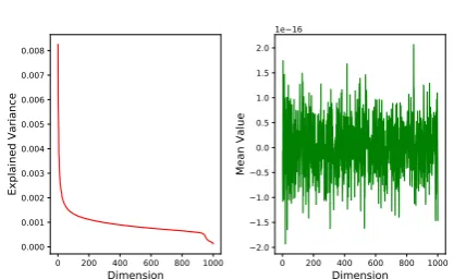
Figure 2: Left: explained variance drops sharply after the top 100 dimensions. Right: all the 1,000 dimen-sions have roughly the same mean value.
using PCA, so that each new dimension repre-sents a principal component. We show that the ex-plained variance goes drastically down for dimen-sions beyond the 100th and stays relatively stable for 100th-1,000th dimensions. In terms of magni-tude, the first dimension explains 69.2 times more variance than the last dimension.
While different dimensions contribute differ-ently to the explained variance, they nonetheless contribute equally to the calculation of inner prod-uct (Figure2, right). Therefore, the lesser dimen-sions, with less variance but equal weighting, ef-fectively decreases the discriminative power of the model. Removing these lesser dimensions enables us to focus on the more discriminative dimensions. To identify optimal dimensionality, beyond which all dimensions are considered lesser, we turn to ex-periments in Section4.
4 Experiments
Given the popularity of the word2vec model
(Mikolov et al.,2013b), we use Skip-gram as the
embedding algorithm. Following Yin and Shen (2018) and Grave et al. (2017), we use the widely
used benchmark datasets, Text8 (Mahoney,2011) and WikiText-103 (Merity et al., 2017), as the training datasets. For ground truth, we train 20 embeddings, with dimensions ranging from 50 to 1,000 at an interval of 50 as well as two embed-dings with dimensions of 5 and 25.2 Here we have made the implicit assumption that 1,000 is an up-per bound for the embedding space’s dimension-ality. For each embedding, we train 200 epochs (Pennington et al.,2014;Shazeer et al.,2016) and keep only the checkpoint that performs best on the word analogy task (Mikolov et al.,2013a). Our experiments focus on (1) comparing our method with grid-search based ground truth and (2) exam-ining consistency between different upper bounds.
4.1 Performance Compared with Grid Search
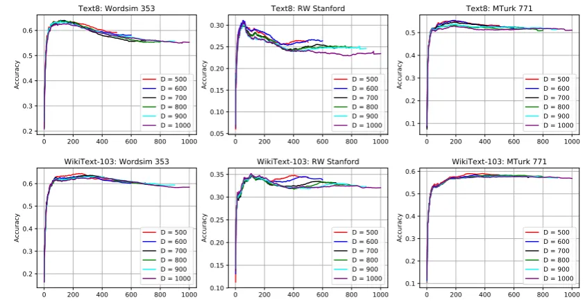
In this subsection, we compare the optimal di-mensionality that our method calculates with the ground truth (Figure 3). We perform the com-parison across three testing datasets: Wordsim 353 (Finkelstein et al., 2002), RW Stanford (
Lu-ong et al., 2013) and MTurk 771 (Halawi et al.,
2012). Figure3demonstrates that our PCA based method (with one training only) is able to uncover the optimal dimensionality. Table 1 reports the distance in selected dimensionalities.
We also observe that the optimal embedding that results from our method (with retraining) is competitive against the optimal embedding found using grid search. In Figure 3, we mark out the respective optimal performances of the two ap-proaches in similarity tasks. In Table2, we further
2
0 200 400 600 800 1000 0.35
0.40 0.45 0.50 0.55 0.60 0.65
Text8: Wordsim 353
Grid Search Our Method
0 200 400 600 800 1000 0.15
0.20 0.25 0.30 0.35
Text8: RW Stanford
Grid Search Our Method
0 200 400 600 800 1000 0.20
0.25 0.30 0.35 0.40 0.45 0.50 0.55
0.60 Text8: MTurk 771
Grid Search Our Method
0 200 400 600 800 1000 0.35
0.40 0.45 0.50 0.55 0.60 0.65
WikiText-103: Wordsim 353
Grid Search Our Method
0 200 400 600 800 1000 0.20
0.25 0.30 0.35 0.40
WikiText-103: RW Stanford
Grid Search Our Method
0 200 400 600 800 1000 0.30
0.35 0.40 0.45 0.50 0.55 0.60
WikiText-103: MTurk 771
[image:4.595.84.504.72.289.2]Grid Search Our Method
Figure 3: Across different benchmarks and different training datasets, the optimal dimensionality that our method (blue curve) identifies closely matches grid search (red curve). The top row is based on Text8. The bottom row is based on WikiText-103. The vertical dotted lines represent the optimal dimensionality for the respective curves. The horizontal dotted line represents the performance of grid search and the blue star marks the performance of our method. The score function isf(i, metric)= metric-50×i. All the curves are averaged over 5 random runs.
0 200 400 600 800 1000 0.2
0.3 0.4 0.5 0.6
Accuracy
Text8: Wordsim 353
D = 500 D = 600 D = 700 D = 800 D = 900 D = 1000
0 200 400 600 800 1000 0.05
0.10 0.15 0.20 0.25 0.30
Accuracy
Text8: RW Stanford
D = 500 D = 600 D = 700 D = 800 D = 900 D = 1000
0 200 400 600 800 1000 0.1
0.2 0.3 0.4 0.5
Accuracy
Text8: MTurk 771
D = 500 D = 600 D = 700 D = 800 D = 900 D = 1000
0 200 400 600 800 1000 0.2
0.3 0.4 0.5 0.6
Accuracy
WikiText-103: Wordsim 353
D = 500 D = 600 D = 700 D = 800 D = 900 D = 1000
0 200 400 600 800 1000 0.10
0.15 0.20 0.25 0.30 0.35
Accuracy
WikiText-103: RW Stanford
D = 500 D = 600 D = 700 D = 800 D = 900 D = 1000
0 200 400 600 800 1000 0.1
0.2 0.3 0.4 0.5 0.6
Accuracy
WikiText-103: MTurk 771
D = 500 D = 600 D = 700 D = 800 D = 900 D = 1000
Figure 4: Across different benchmarks and different training datasets, consistency is observed when the upper bound is set to 500, 600, 700, 800, 900 and 1,000. The curves trace closely each other, in particular for WordSim 353 and MTurk 771. The top row is based on the Text8 dataset. The bottom row is based on the WikiText-103 dataset. All the curves are averaged over 5 random runs. Best viewed in color.
report the optimal performance achieved by grid search and our method as well as their relative per-formance. Even though we have only trained one embedding (and one retraining), our method, on average, is able to achieve 100.2% (WordSim 353) to 96.9% (MTurk 771) of the optimal performance
by grid-searching through 22 sets of embeddings.
4.2 Consistency across Upper Bounds
[image:4.595.85.507.381.599.2]Table 1: Distance in Dimensionalities between Grid Search and Our Proposed Method (Numbers within the bucket size 50 are in bold)
Datasets WordSim RW Stanford MTurk
Text8 34 1 65
WikiText 18 10 48
[image:5.595.72.291.107.165.2]Average 26 5.5 66.5
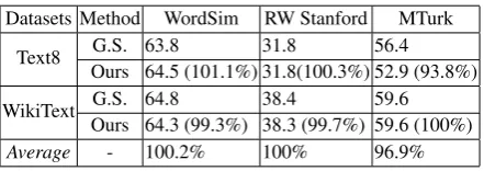
Table 2: Performance (Correlation) Comparison be-tween Grid Search and Our Proposed Method
Datasets Method WordSim RW Stanford MTurk
Text8 G.S. 63.8 31.8 56.4
Ours 64.5 (101.1%) 31.8(100.3%) 52.9 (93.8%)
WikiText G.S. 64.8 38.4 59.6
Ours 64.3 (99.3%) 38.3 (99.7%) 59.6 (100%)
Average - 100.2% 100% 96.9%
subsection, we demonstrate our method is robust against different upper bounds.
In Figure 4, we vary the dimension from 500 to 1,000 at an increment of 100. We observe that the dimensionality our method selects is consis-tent across different upper bounds. Based on the demonstrated consistency, different upper bounds can be selected and still the optimal dimensional-ity can be uncovered as long as the chosen upper bound is larger than the optimal dimensionality.
4.3 Efficiency Compared with Grid Search
In this subsection, we report the running time of our algorithm and compare it with that of grid search. We have recorded the running time of our experiments and that of the PCA transformations. We average them over 5 random runs (Figure5).
For Text8, grid search takes 22,801 minutes cu-mulatively. Training a 1,000-dimension embed-ding takes 1,724 minutes. The PCA step takes 22 minutes (note that for each embedding we only need one PCA operation). This represents a 13.1x speedup for our method. For WikiText-103, grid search takes 132,652 minutes. Training a 1,000-dimension embedding takes 10,448 minutes. The PCA step takes 34 minutes. This represents a 12.7x speedup.
We note that the comparison results are depen-dent on grid granularity. A coarser grid search could save researchers more time, at the cost of performance loss.
0 200 400 600 800 1000
# Dimension
400 600 800 1000 1200 1400 1600 1800
Training Time (mins)
Text8
0 200 400 600 800 1000
# Dimension
2000 4000 6000 8000 10000
Training Time (mins)
WikiText-103
Figure 5: Left: training time for Text8 for embeddings of different dimensions for 200 epochs using 6 CPUs. Right: training time for WikiText-103 for embeddings of different dimensions for 200 epochs using 10 CPUs. All results are averaged over 5 random runs.
5 Conclusion
In this paper, we provided a fast and reliable method based on PCA to select the number of di-mensions for training word embeddings. First, we train one embedding with a generous upper bound (e.g. 1,000) of dimensions. Then we transform the embedding using PCA and incrementally re-move the lesser dimensions while recording the embeddings’ performance on language tasks. Ex-periments demonstrate that (1) our method is able to identify the optimal dimensionality, (2) the re-sulting embedding has competitive performance against grid search, and (3) our method is robust against the selection of the upper bound.
Acknowledgement
The authors would like to thank Hang Zhao and Srinivasan Venkatachary for supporting this project, would like to thank Russ Webb, Arnab Ghoshal, and Jaewook Chung for their insight-ful comments on early versions of this paper, and would like to thank the anonymous EMNLP-IJCNLP reviewers for their reviews and sugges-tions.
References
Christopher M. Bishop. 2006. Pattern Recognition and Machine Learning. Springer.
[image:5.595.72.293.215.293.2]Jacob Devlin, Ming-Wei Chang, Kenton Lee, and Kristina Toutanova. 2018. Bert: Pre-training of deep bidirectional transformers for language understand-ing. arXiv preprint.
Manaal Faruqui, Yulia Tsvetkov, Dani Yogatama, Chris Dyer, and Noah A. Smith. 2015. Sparse over-complete word vector representations. Proceedings of the 53rd Annual Meeting of the Association for Computational Linguistics, pages 1491–1500.
Lev Finkelstein, Evgeniy Gabrilovich, Yossi Matias, Ehud Rivlin, Gadi Wolfman Zach Solan, and Eytan Ruppin. 2002. Placing search in context: the con-cept revisited. ACM Transactions on Information Systems, 20(1):116–131.
Edouard Grave, Armand Joulin, and Nicolas Usunier. 2017. Improving neural language models with a continuous cache. ICLR 2017.
Guy Halawi, Gideon Dror, Evgeniy Gabrilovich, and Yehuda Koren. 2012. Large-scale larning of word relatedness with constraints. KDD.
Matt J. Kusner, Yu Sun, Nicholas I. Kolkin, and Kil-ian Q. Weinberger. 2015. From Word Embeddings To Document Distances. Proceedings of the 32 nd International Conference on Machine Learning.
Siwei Lai, Kang Liu, Shizhu He, and Jun Zhao. 2016. How to generate a good word embedding. IEEE In-telligent Systems, 31(6).
Yiou Lin, Hang Lei, Jia Wu, and Xiaoyu Li. 2015. An Empirical Study on Sentiment Classification of Chinese Review using Word Embedding. 29th Pa-cific Asia Conference on Language, Information and Computation, pages 258 – 266.
Shaoshi Ling, Yangqiu Song, and Dan Roth. 2016. Word embeddings with limited memory. Proceed-ings of the 54th Annual Meeting of the Association for Computational Linguistics, pages 387–392.
Thang Luong, Richard Socher, and Christopher Man-ning. 2013. Better word representations with re-cursive neural networks for morphology. Proceed-ings of the Seventeenth Conference on Computa-tional Natural Language Learning.
Matt Mahoney. 2011. Large text compression bench-mark.
Stephen Merity, Caiming Xiong, James Bradbury, and Richard Socher. 2017. Pointer sentinel mixture models. ICLR 2017.
Tomas Mikolov, Kai Chen, Greg Corrado, and Jeffrey Dean. 2013a. Efficient Estimation of Word Repre-sentations in Vector Space. ICLR Workshop.
Tomas Mikolov, Ilya Sutskever, Kai Chen, Greg Cor-rado, and Jeffrey Dean. 2013b. Distributed Repre-sentations of Words and Phrases and their Composi-tionality. NIPS’13 Proceedings of the 26th Interna-tional Conference on Neural Information Processing Systems, 2:3111–3119.
Andriy Mnih and Koray Kavukcuoglu. 2013. Learning word embeddings efficiently with noise-contrastive estimation. NIPS’13 Proceedings of the 26th In-ternational Conference on Neural Information Pro-cessing Systems, 2.
Jiaqi Mu and Pramod Viswanath. 2018. All-but-the-top: Simple and effective postprocessing for word representations. Sixth International Conference on Learning Representations (ICLR 2018).
Maximillian Nickel and Douwe Kiela. 2017. Poincar´e embeddings for learning hierarchical representa-tions. Advances in Neural Information Processing Systems 30 (NIPS 2017).
Jeffrey Pennington, Richard Socher, and Christo-pher D. Manning. 2014. GloVe: Global Vectors for Word Representation. InEmpirical Methods in Nat-ural Language Processing (EMNLP), pages 1532– 1543.
Bryan Perozzi, Rami Al-Rfou, and Steven Skiena. 2014.DeepWalk: Online Learning of Social Repre-sentations. KDD ’14 Proceedings of the 20th ACM SIGKDD International Conference on Knowledge Discovery and Data Mining, pages 701–210.
Vikas Raunak. 2017. Simple and effective dimension-ality reduction for word embeddings. Advances in Neural Information Processing Systems 30 (NIPS 2017) LLD Workshop.
Noam Shazeer, Ryan Doherty, Colin Evans, and Chris Waterson. 2016. Swivel: Improv-ing EmbeddImprov-ings by NoticImprov-ing What’s MissImprov-ing.
https://arxiv.org/abs/1602.02215.
Raphael Shu and Hideki Nakayama. 2018. Compress-ing word embeddCompress-ings via deep compositional code learning.ICLR 2018 Conference.
Jian Tang, Meng Qu, Mingzhe Wang, Ming Zhang, Jun Yan, and Qiaozhu Mei. 2015. LINE: Large-scale Information Network Embedding. Interna-tional World Wide Web Conference.
Lei Tang and Huan Liu. 2009. Relational learning via latent social dimensions. KDD ’09: Proceedings of the 15th ACM SIGKDD International Conference on Knowledge Discovery and Data Mining.
Yu Wang, Yang Feng, Zhe Hong Ryan Berger, and Jiebo Luo. 2017. How Polarized Have We Be-come? A Multimodal Classification of Trump Fol-lowers and Clinton FolFol-lowers.SocInfo 2017: Social Informatics, pages 440–456.
Junting Ye, Shuchu Han, Yifan Hu, Baris Coskun, Meizhu Liu, Hong Qin, and Steven Skiena. 2017. Nationality Classification Using Name Embeddings.
CIKM’17, pages 1897–1906.