Proceedings of the 2016 Conference on Empirical Methods in Natural Language Processing, pages 287–296,
Semi-Supervised Learning of Sequence Models with the Method of Moments
Zita Marinho∗] Andr´e F. T. Martins†♥♦ Shay B. Cohen♣ Noah A. Smith♠ ∗Instituto de Sistemas e Rob´otica, Instituto Superior T´ecnico, 1049-001 Lisboa, Portugal†Instituto de Telecomunicac¸˜oes, Instituto Superior T´ecnico, 1049-001 Lisboa, Portugal ]School of Computer Science, Carnegie Mellon University, Pittsburgh, PA 15213, USA
♥Unbabel Lda, Rua Visconde de Santar´em, 67-B, 1000-286 Lisboa, Portugal ♦Priberam Labs, Alameda D. Afonso Henriques, 41, 2o, 1000-123 Lisboa, Portugal
♣School of Informatics, University of Edinburgh, Edinburgh EH8 9AB, UK ♠Computer Science & Engineering, University of Washington, Seattle, WA 98195, USA
[email protected],[email protected], [email protected],[email protected]
Abstract
We propose a fast and scalable method for semi-supervised learning of sequence models, based on anchor words and moment matching. Our method can handle hidden Markov mod-els with feature-based log-linear emissions. Unlike other semi-supervised methods, no de-coding passes are necessary on the unlabeled data and no graph needs to be constructed— only one pass is necessary to collect moment statistics. The model parameters are estimated by solving a small quadratic program for each feature. Experiments on part-of-speech (POS) tagging for Twitter and for a low-resource lan-guage (Malagasy) show that our method can learn from very few annotated sentences.
1 Introduction
Statistical learning of NLP models is often lim-ited by the scarcity of annotated data. Weakly su-pervised methods have been proposed as an alter-native to laborious manual annotation, combining large amounts of unlabeled data with limited re-sources, such as tag dictionaries or small annotated datasets (Merialdo, 1994; Smith and Eisner, 2005; Garrette et al., 2013). Unfortunately, most semi-supervised learning algorithms for the structured problems found in NLP are computationally expen-sive, requiring multiple decoding passes through the unlabeled data, or expensive similarity graphs. More scalable learning algorithms are in demand.
In this paper, we propose a moment-matching method for semi-supervised learning of sequence models. Spectral learning and moment-matching approaches have recently proved a viable alternative
to expectation-maximization (EM) for unsupervised learning (Hsu et al., 2012; Balle and Mohri, 2012; Bailly et al., 2013), supervised learning with latent variables (Cohen and Collins, 2014; Quattoni et al., 2014; Stratos et al., 2013) and topic modeling (Arora et al., 2013; Nguyen et al., 2015). These methods have learnability guarantees, do not suffer from lo-cal optima, and are computationally less demanding. Unlike spectral methods, ours does not require an orthogonal decomposition of any matrix or tensor. Instead, it considers a more restricted form of super-vision: words that have unambiguous annotations, so-calledanchor words(Arora et al., 2013). Rather than identifying anchor words from unlabeled data (Stratos et al., 2016), we extract them from a small labeled dataset or from a dictionary. Given the an-chor words, the estimation of the model parameters can be made efficient by collecting moment statistics from unlabeled data, then solving a small quadratic program for each word.
Our contributions are as follows:
• We adapt anchor methods to semi-supervised
learning of generative sequence models.
• We show how our method can also handle
log-linear feature-based emissions.
• We apply this model to POS tagging. Our
ex-periments on the Twitter dataset introduced by Gimpel et al. (2011) and on the dataset in-troduced by Garrette et al. (2013) for Mala-gasy, a low-resource language, show that our method does particularly well with very little la-beled data, outperforming semi-supervised EM and self-training.
2 Sequence Labeling
In this paper, we address the problem of sequence labeling. Letx1:L=hx1, . . . , xLibe a sequence of Linput observations (for example, words in a
sen-tence). The goal is to predict a sequence of labels h1:L=hh1, . . . , hLi, where eachhiis a label for the observationxi (for example, the word’s POS tag).
We start by describing two generative sequence models: hidden Markov models (HMMs,§2.1), and their generalization with emission features (§2.2). Later, we propose a weakly-supervised method for estimating these models’ parameters (§3–§4) based only on observed statistics of words and contexts.
2.1 Hidden Markov Models
We define random variables X := hX1, . . . , XLi andH :=hH1, . . . , HLi, corresponding to observa-tions and labels, respectively. EachXi is a random variable over a setX (the vocabulary), and eachHi ranges overH (a finite set of “states” or “labels”). We denote the vocabulary size byV =|X |, and the number of labels byK = |H|. A first-order HMM has the following generative scheme:
p(X =x1:L,H =h1:L) := (1) L
Y
`=1
p(X`=x` |H`=h`) L
Q
`=0
p(H`+1=h`+1 |H`=h`),
where we have defined h0 = START and hL+1 =
STOP. We adopt the following notation for the pa-rameters:
• The emission matrix O ∈ RV×K, defined as
Ox,h:=p(X` =x|H`=h),∀h∈ H, x∈ X.
• The transition matrixT ∈ R(K+2)×(K+2), de-fined asTh,h0 := p(H`+1 = h | H` = h0), for everyh, h0 ∈ H ∪ {START,STOP}. This matrix satisfiesT>1=1.1
Throughout the rest of the paper we will adopt
X ≡ X` andH ≡ H` to simplify notation, when-ever the index ` is clear from the context. Under
this generative process, predicting the most proba-ble label sequence h1:L given observations x1:L is
1That is, it satisfies PK
h=1p(H`+1 = h | H` = h0) + p(H`+1 = STOP|H` =h0) = 1; and alsoPKh=1p(H1 =
h|H0=START) = 1.
accomplished with the Viterbi algorithm inO(LK2) time.
If labeled data are available, the model param-eters O and T can be estimated with the maxi-mum likelihood principle, which boils down to a simple counting of events and normalization. If we only have unlabeled data, the traditional ap-proach is the expectation-maximization (EM) algo-rithm, which alternately decodes the unlabeled ex-amples and updates the model parameters, requiring multiple passes over the data. The same algorithm can be used in semi-supervised learning when la-beled and unlala-beled data are combined, by initial-izing the model parameters with the supervised esti-mates and interpolating the estiesti-mates in the M-step.
2.2 Feature-Based Hidden Markov Models
Sequence models with log-linear emissions have been considered by Smith and Eisner (2005), in a discriminative setting, and by Berg-Kirkpatrick et al. (2010), as generative models for POS induc-tion. Feature-based HMMs (FHMMs) define a fea-ture function for words,φ(X)∈RW, which can be discrete or continuous. This allows, for example, to indicate whether an observation, corresponding to a word, starts with an uppercase letter, contains digits or has specific affixes. More generally, it helps with the treatment of out-of-vocabulary words. The emis-sion probabilities are modeled asKconditional
dis-tributions parametrized by a log-linear model, where theθh∈RW represent feature weights:
p(X=x|H =h) := exp(θh>φ(x))/Z(θh). (2)
Above, Z(θh) := Px0∈Xexp(θ>hφ(x0)) is a nor-malization factor. We will show in §4 how our
moment-based semi-supervised method can also be used to learn the feature weightsθh.
3 Semi-Supervised Learning via Moments We now describe our moment-based semi-supervised learning method for HMMs. Through-out, we assume the availability of a small labeled datasetDLand a large unlabeled datasetDU.
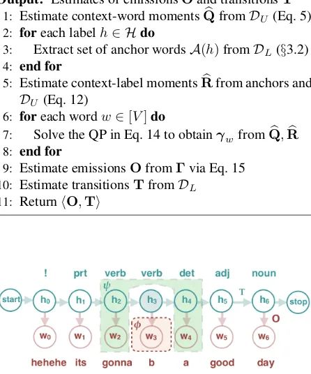
Algorithm 1Semi-Supervised Learning of HMMs with Moments
Input: Labeled datasetDL, unlabeled datasetDU Output: Estimates of emissionsOand transitionsT
1: Estimate context-word momentsQb fromDU (Eq. 5) 2: foreach labelh∈ Hdo
3: Extract set of anchor wordsA(h)fromDL(§3.2) 4: end for
5: Estimate context-label momentsRbfrom anchors and
DU (Eq. 12)
6: foreach wordw∈[V]do
7: Solve the QP in Eq. 14 to obtainγwfromQb,Rb 8: end for
9: Estimate emissionsOfromΓvia Eq. 15
[image:3.612.75.298.102.370.2]10: Estimate transitionsTfromDL 11: ReturnhO,Ti
Figure 1: HMM, context (green) conditionally indepen-dent of present (red)w`given stateh`.
and will be formally defined in §3.1. Such
co-occurrence matrices are often collected in NLP, for various problems, ranging from dimensionality re-duction of documents using latent semantic index-ing (Deerwester et al., 1990; Landauer et al., 1998), distributional semantics (Sch¨utze, 1998; Levy et al., 2015) and word embedding generation (Dhillon et al., 2015; Osborne et al., 2016). We can build such a moment matrix entirely from the unlabeled dataDU. The same unlabeled data is used to build an estimate of acontext-label moment matrixR ∈RC×K, as explained in§3.3. This is done by first identifying words that are unambiguously associated with each labelh, calledanchor words, with the aid of a few
labeled data; this is outlined in§3.2. Finally, given empirical estimates of Q and R, we estimate the emission matrixOby solving a small optimization problem independently per word (§3.4). The transi-tion matrixTis obtained directly from the labeled datasetDLby maximizing the likelihood.
3.1 Moments of Contexts and Words
To formalize the notion of “context,” we introduce the shorthandZ` := hX1:(`−1),X(`+1):Li. Impor-tantly, the HMM in Eq. 1 entails the following con-ditional independence assumption:X`is condition-ally independent of the surrounding contextZ`given the hidden stateH`. This is illustrated in Figure 1, using POS tagging as an example task.
We introduce a vector of context features ψ(Z`) ∈ RC, which may look arbitrarily within the context Z` (left or right), but not at X` itself. These features could be “one-hot” representations or other reduced-dimensionality embeddings (as de-scribed later in§5). Consider the word w ∈ X an
instance ofX ≡X`. A pivotal matrix in our formu-lation is the matrixQ∈RC×V, defined as:
Qc,w :=E[ψc(Z)|X =w]. (3)
Expectations here are taken with respect to the prob-abilistic model in Eq. 1 that generates the data. The following quantities will also be necessary:
qc:=E[ψc(Z)], pw :=p(X =w). (4)
Since all the variables in Eqs. 3–4 are observed, we can easily obtain empirical estimates by taking ex-pectations over the unlabeled data:
b
Qc,w =
P
x,Pz∈DUψc(z)1(x=w) x,z∈DU1(x=w)
, (5)
b
qc = Px,z∈DUψc(z)
.
|DU|, (6)
b
pw = Px,z∈DU1(x=w)
.
|DU|. (7)
where we take1(x=w)to be the indicator for word
w. Note that, under our modeling assumptions, Q decomposes in terms of its hidden states:
E[ψc(Z)|X=w] = (8)
X
h∈H
p(H =h|X=w)E[ψc(Z)|H=h]
The reason why this holds is that, as stated above,Z andXare conditionally independent givenH.
3.2 Anchor Words
state is assumed to be deterministic, regardless of context. In this work, we generalize this notion to more than one anchor word per label, for improved context estimates. This allows for more flexible forms of anchors with weak supervision. For each stateh∈ H, let its set of anchor words be
A(h)={w∈ X :p(H =h|X =w) = 1} (9) =w∈ X :Ow,h>0∧Ow,h0=0,∀h06=h .
That is,A(h)is the set of unambiguous words that always take the labelh. This can be estimated from
the labeled dataset DL by collecting the most fre-quent unambiguous words for each label.
Algorithms for identifyingA(h) from unlabeled data alone were proposed by Arora et al. (2013) and Zhou et al. (2014), with application to topic models. Our work differs in which we do not aim to discover anchor words from pure unlabeled data, but rather exploit the fact that small amounts of labeled data are commonly available in many NLP tasks—better anchors can be extracted easily from such small la-beled datasets. In §5 we give a more detailed de-scription of the selection process.
3.3 Moments of Contexts and Labels
We define the matrixR∈RC×K as follows:
Rc,h:=E[ψc(Z)|H=h]. (10)
Since the expectation in Eq. 10 is conditioned on the (unobserved) labelh, we cannot directly estimate it
using moments of observed variables, as we do for Q. However, if we have identified sets of anchor words for each labelh∈ H, we have:
E[ψc(Z)|X∈ A(h)] = = X
h0
E[ψc(Z)|H =h0]p(H=h0 |X∈ A(h))
| {z }
=1(h0=h)
= Rc,h. (11)
Therefore, given the set of anchor wordsA(h), the hth column of Rcan be estimated in a single pass over the unlabeled data, as follows:
b
Rc,h=
P
x,Pz∈DUψc(z)1(x∈ A(h)) x,z∈DU1(x∈ A(h))
(12)
3.4 Emission Distributions
We can now put all the ingredients above together to estimate the emission probability matrixO. The procedure we propose here is computationally very efficient, since only one pass is required over the un-labeled data, to collect the co-occurrence statisticsQb
andRb. The emissions will be estimated from these
moments by solving a small problem independently for each word. Unlike EM and self-training, no de-coding is necessary, only counting and normalizing; and unlike label propagation methods, there is re-quirement to build a graph with the unlabeled data.
The crux of our method is the decomposition in Eq. 8, which is combined with the one-to-one cor-respondence between labels h and anchor words
A(h). We can rewrite Eq. 8 as:
Qc,w =
X
h
Rc,h p(H =h|X=w). (13)
In matrix notation, we haveQ = RΓ, whereΓ ∈
RK×V is defined asΓ
h,w :=p(H =h|X =w). If we had infinite unlabeled data, our moment es-timates Qb and Rb would be perfect and we could solve the system of equations in Eq. 13 to obtain Γ exactly. Since we have finite data, we resort to a least squares solution. This corresponds to solv-ing a simple quadratic program (QP) per word, in-dependent from all the other words, as follows. De-note by qw := E[ψ(Z) | X = w] ∈ RC and by
γw:=p(H=· |X=w) ∈ RKthewth columns ofQandΓ, respectively. We estimate the latter dis-tribution following Arora et al. (2013):
b
γw = arg min
γw kqw−Rγwk
2 2
s.t. 1>γw = 1, γw≥0.
(14)
Note that this QP is very small—it has only K
variables—hence, we can solve it very quickly (1.7 ms on average, in Gurobi, withK = 12).
Given the probability tables forp(H = h |X = w), we can estimate the emission probabilitiesOby direct application of Bayes rule:
b
Ow,h=
p(H=h|X=w)×p(X =w) p(H=h) (15)
= bγw,c× Eq. 7
z}|{ b
pw
P
These parameters are guaranteed to lie in the prob-ability simplex, avoiding the need of heuristics for dealing with “negative” and “unnormalized” prob-abilities required by prior work in spectral learn-ing (Cohen et al., 2013).
3.5 Transition Distributions
It remains to estimate the transition matrix T. For the problems tackled in this paper, the number of labelsK is small, compared to the vocabulary size V. The transition matrix has onlyO(K2)degrees of freedom, and we found it effective to estimate it us-ing the labeled sequences inDLalone, without any refinement. This was done by smoothed maximum likelihood estimation on the labeled data, which boils down to counting occurrences of consecutive labels, applying add-one smoothing to avoid zero probabilities for unobserved transitions, and normal-izing.
For problems with numerous labels, a possible al-ternative is the composite likelihood method (Cha-ganty and Liang, 2014). GivenOb, the maximization
of the composite log-likelihood function leads to a convex optimization problem that can be efficiently optimized with an EM algorithm. A similar proce-dure was carried out by Cohen and Collins (2014).2
4 Feature-Based Emissions
Next, we extend our method to estimate the param-eters of the FHMM in §2.2. Other than contextual features ψ(Z) ∈ RC, we also assume a feature encoding function for words, φ(X) ∈ RW. Our framework, illustrated in Algorithm 2, allows for both discrete and continuous word and context fea-tures. Lines 2–5 are the same as in Algorithm 1, replacing word occurrences with expected values of word features (we redefine Q and Γ to cope with features instead of words). The main difference with respect to Algorithm 1 is that we do not es-timate emission probabilities; rather, we first esti-mate the mean parameters (feature expectations E[φ(X) | H = h]), by solving one QP for each
2In preliminary experiments, the compositional likelihood
method was not competitive with estimating the transition ma-trices directly from the labeled data, on the datasets described in§6; results are omitted due to lack of space. However, this may be a viable alternative if there is no labeled data and the anchors are extracted from gazetteers or a dictionary.
Algorithm 2 Semi-Supervised Learning of Feature-Based HMMs with Moments
Input: Labeled datasetDL, unlabeled datasetDU Output: Emission log-linear parametersΘ and
transi-tionsT
1: Estimate context-word moments Qb from DU (Eq. 20)
2: foreach labelh∈ Hdo
3: Extract set of anchor wordsA(h)fromDL(§3.2) 4: end for
5: Estimate context-label momentsRb from the anchors andDU (Eq. 12)
6: foreach word featurej∈[W]do
7: Solve the QP in Eq. 22 to obtainγjfromQb,Rb 8: end for
9: foreach labelh∈ Hdo
10: Estimate the mean parametersµhfromΓ(Eq. 24) 11: Estimate the canonical parametersθhfromµhby
solving Eq. 25 12: end for
13: Estimate transitionsTfromDL 14: ReturnhΘ,Ti
emission feature; and then we solve a convex op-timization problem, for each label h, to recover
the log-linear weights over emission features (called
canonical parameters).
4.1 Estimation of Mean Parameters
First of all, we replace word probabilities by expec-tations over word features. We redefine the matrix Γ∈RK×W as follows:
Γh,j :=
p(H =h)×E[φj(X)|H=h] E[φj(X)]
. (17)
Note that, with one-hot word features, we have E[φw(X) | H = h] = P(X = w | H = h), E[φw(X)] = p(X = w), and therefore Γh,w = p(H = h | X = w), so this can be regarded as a generalization of the framework in§3.4.
Second, we redefine the context-word moment matrixQas the following matrix inRC×W:
Qc,j = E[ψc(Z)×φj(X)]/E[φj(X)]. (18)
Again, note that we recover the previousQif we use one-hot word features. We then have the following generalization of Eq. 13:
E[ψc(Z)×φj(X)]/E[φj(X)] = (19)
P
or, in matrix notation,Q=RΓ.
Again, matricesQandRcan be estimated from data by collecting empirical feature expectations over unlabeled sequences of observations. For R use Eq. 12 with no change; forQreplace Eq. 5 by
b
Qc,j = Px,z∈DUψc(z)φj(x)
. P
x,z∈DUφj(x).(20)
Letqj ∈RC andγj ∈RKbe columns ofQb andΓb, respectively. Note that we must have
1>γj =X h
P(H=h)E[φj(X)|H=h]
E[φj(X)] = 1, (21)
since E[φj(X)] = PhP(H = h)E[φj(X)|H=h]. We rewrite the QP to minimize the squared difference for each dimension
jindependently:
b
γj = arg min
γj
qj−Rγj
2
2 s.t. 1>γj = 1.
(22) Note that, ifφ(x) ≥0for allx∈ X, then we must
haveγj ≥0, and therefore we may impose this in-equality as an additional constraint.
Letγ¯ ∈ RK be the vector of state probabilities, with entries¯γh :=p(H =h)forh ∈ H. This vec-tor can also be recovered from the unlabeled dataset and the set of anchors, by solving another QP that aggregates information for all words:
¯
γ = arg min
¯
γ kq¯−Rγ¯k
2
2 s.t. 1>γ¯ = 1, γ¯ ≥0.
(23) where q¯ := Eb[ψ(Z)] ∈ RC is the vector whose entries are defined in Eq. 6.
Let µh := E[φ(X) | H = h] ∈ RW be the mean parameters of the distribution for each stateh. These parameters are computed by solvingW
inde-pendent QPs (Eq. 22), yielding the matrixΓdefined in Eq. 17, and then applying the formula:
µh,j = Γj,h×E[φj(X)]/ ¯γh, (24)
withγ¯h=p(H =h)estimated as in Eq. 23.
4.2 Estimation of Canonical Parameters
To compute a mapping from mean parameters µh to canonical parametersθh, we use the well-known Fenchel-Legendre duality between the entropy and the log-partition function (Wainwright and Jordan,
2008). Namely, we need to solve the following con-vex optimization problem:
b
θh = arg max
θh
θ>hµh−logZ(θh) +kθhk, (25)
where is a regularization constant.3 In practice,
this regularization is important, since it preventsθh from growing unbounded wheneverµhfalls outside the marginal polytope of possible mean parameters. We solve Eq. 25 with the limited-memory BFGS al-gorithm (Liu and Nocedal, 1989).
5 Method Improvements
In this section we detail three improvements to our moment-based method that had a practical impact.
Supervised Regularization. We add a supervised penalty term to Eq. 22 to keep the label posteriorsγj close to the label posteriors estimated in the labeled set,γ0j, for every featurej ∈[W]. The regularized least-squares problem becomes:
min
γj
(1−λ)kqj −Rγjk2+λkγj−γ0jk2
s.t. 1>γj = 1. (26)
CCA Projections. A one-hot feature representa-tion of words and contexts has the disadvantage that it grows with the vocabulary size, making the mo-ment matrixQ too sparse. The number of contex-tual features and words can grow rapidly on large text corpora. Similarly to Cohen and Collins (2014) and Dhillon et al. (2015), we use canonical correla-tion analysis (CCA) to reduce the dimension of these vectors. We use CCA to form low-dimensional pro-jection matrices for features of wordsPW ∈RW×D and features of contextsPC ∈ RC×D, withD min{W, C}. We use these projections on the origi-nal feature vectors and replace the these vectors with their projections.
Selecting Anchors. We collect counts of each word-label pair, and select up to 500 anchors with high conditional probability on the anchoring state
b
p(h | w). We tuned the probability threshold to
3As shown by Xiaojin Zhu (1999) and Yasemin Altun
select the anchors on the validation set, using steps of 0.1 in the unit interval, and making sure that all tags have at least one anchor. We also considered a frequency threshold, constraining anchors to oc-cur more than 500 times in the unlabeled corpus, and four times in the labeled corpus. Note that past work used a single anchor word per state (i.e.,
|A(h)|= 1). We found that much better results are obtained when |A(h)| 1, as choosing more an-chors increases the number of samples used to esti-mate the context-label moment matrixRb, reducing
noise.
6 Experiments
We evaluated our method on two tasks: POS tagging of Twitter text (in English), and POS tagging for a low-resource language (Malagasy). For all the ex-periments, we used the universal POS tagset (Petrov et al., 2012), which consists of K = 12 tags. We compared our method against supervised base-lines (HMM and FHMM), which use the labeled data only, and two semi-supervised baselines that exploit the unlabeled data: self-training and EM. For the Twitter experiments, we also evaluated a stacked architecture in which we derived features from our model’s predictions to improve a state-of-the-art POS tagger (MEMM).4
6.1 Twitter POS Tagging
For the Twitter experiment, we used the Oct27 dataset of Gimpel et al. (2011), with the provided partitions (1,000 tweets for training and 328 for val-idation), and tested on the Daily547 dataset (547 tweets). Anchor words were selected from the train-ing partition as described in §5. We used 2.7M unlabeled tweets (O’Connor et al., 2010) to train the semi-supervised methods, filtering the English tweets as in Lui and Baldwin (2012), tokenizing them as in Owoputi et al. (2013), and normalizing at-mentions, URLs, and emoticons.
We used as word features φ(X) the word iself, as well as binary features for capitalization, titles, and digits (Berg-Kirkpatrick et al., 2010), the word shape, and the Unicode class of each character. Sim-ilarly to Owoputi et al. (2013), we also used suf-fixes and presuf-fixes (up to length 3), and
Twitter-4http://www.ark.cs.cmu.edu/TweetNLP/
0.7 0.75 0.8 0.85 0.9 0.95
0 100 200 300 400 500 600 700 800 900 1000
Tag
gi
ng
ac
cu
rac
y (
0/
1 l
os
s)
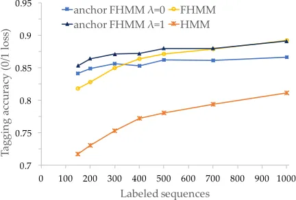
[image:7.612.317.533.63.209.2]Labeled sequences anchor FHMM λ=0 FHMM anchor FHMM λ=1 HMM
Figure 2: POS tagging accuracy in the Twitter data versus the number of labeled training sequences.
specific features: whether the word starts with @, #, orhttp://. As contextual features ψ(Z), we de-rive analogous features for the preceding and fol-lowing words, before reducing dimensionality with CCA. We collect feature expectations for words and contexts that occur more than 20 times in the un-labeled corpus. We tuned hyperparameters on the development set: the supervised interpolation co-efficient in Eq. 26, λ ∈ {0,0.1, . . . ,1.0}, and, for all systems, the regularization coefficient ∈
{0.0001,0.001,0.01,0.1,1,10}. (Underlines indi-cate selected values.) The former controls how much we rely on the supervised vs. unsupervised es-timates. Forλ= 1.0we used supervised estimates only for words that occur in the labeled corpus, all the remaining words rely solely on unsupervised es-timates.
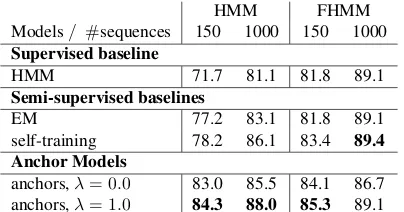
unregular-HMM FHMM Models/ #sequences 150 1000 150 1000 Supervised baseline
HMM 71.7 81.1 81.8 89.1
Semi-supervised baselines
EM 77.2 83.1 81.8 89.1
self-training 78.2 86.1 83.4 89.4 Anchor Models
anchors,λ= 0.0 83.0 85.5 84.1 86.7 anchors,λ= 1.0 84.3 88.0 85.3 89.1 Table 1: Tagging accuracies on Twitter. Shown are the supervised and semi-supervised baselines, and our moment-based method, trained with 150 training labeled sequences, and the full labeled corpus (1000 sequences).
ized model λ = 0.0 relies solely on unsupervised estimates given the set of anchors.
Semi-supervised comparison. Next, we compare our method to two other semi-supervised baselines, using both HMMs and FHMMs: EM and self-training. EM requires decoding and counting in multiple passes over the full unlabeled corpus. We initialized the parameters with the supervised esti-mates, and selected the iteration with the best ac-curacy on the development set.5 The self-training baseline uses the supervised system to tag the unla-beled data, and then retrains on all the data.
Results are shown in Table 1. We observe that, for small amounts of labeled data (150 tweets), our method outperforms all the supervised and semi-supervised baselines, yielding accuracies 6.1 points above the best semi-supervised baseline for a simple HMM, and 1.9 points above for the FHMM. With more labeled data (1,000 instances), our method out-performs all the baselines for the HMM, but not with the more sophisticated FHMM, in which our accura-cies are 0.3 points below the self-training method.6 These results suggest that our method is more effec-tive when the amount of labeled data is small.
5The FHMM with EM did not perform better than the
su-pervised baseline, so we consider the initial value as the best accuracy under this model.
6According to a word-level paired Kolmogorov-Smirnov
test, for the FHMM with 1,000 tweets, the self-training method outperforms the other methods with statistical significance at p <0.01; and for the FHMM with 150 tweets the anchor-based and self-training methods outperform the other baselines with the samep-value. Our best HMM outperforms the other base-lines at a significance level ofp <0.01for 150 and 1000 se-quences.
[image:8.612.74.276.57.163.2]150 1000 MEMM (same+clusters) 89.57 93.36 MEMM (same+clusters+posteriors) 91.14 93.18 MEMM (all+clusters) 91.55 94.17 MEMM (all+clusters+posteriors) 92.06 94.11 Table 2: Tagging accuracy for the MEMM POS tagger of Owoputi et al. (2013) with additional features from our model’s posteriors.
Stacking features. We also evaluated a stacked ar-chitecture in which we use our model’s predictions as an additional feature to improve the state-of-the-art Twitter POS tagger of Owoputi et al. (2013). This system is based on a semi-supervised discriminative model with Brown cluster features (Brown et al., 1992). We provide results using their full set of fea-tures (all), and using the same set of features in our anchor model (same). We compare tagging accuracy on a model with these features plus Brown clusters (+clusters) against a model that also incorporates the posteriors from the anchor method as an addi-tional feature in the MEMM (+clusters+posteriors). The results in Table 2 show that using our model’s posteriors are beneficial in the small labeled case, but not if the entire labeled data is used.
Runtime comparison. The training time of an-chor FHMM is 3.8h (hours), for self-training HMM 10.3h, for EM HMM 14.9h and for Twitter MEMM (all+clusters) 42h. As such, the anchor method is much more efficient than all the baselines because it requires a single pass over the corpus to collect the moment statistics, followed by the QPs, with-out the need to decode the unlabeled data. EM and the Brown clustering method (the latter used to ex-tract features for the Twitter MEMM) require several passes over the data; and the self-training method in-volves decoding the full unlabeled corpus, which is expensive when the corpus is large. Our analysis adds to previous evidence that spectral methods are more scalable than learning algorithms that require inference (Parikh et al., 2012; Cohen et al., 2013).
6.2 Malagasy POS Tagging
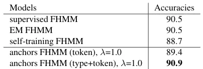
[image:8.612.310.537.60.118.2]Models Accuracies
supervised FHMM 90.5
EM FHMM 90.5
self-training FHMM 88.7
[image:9.612.84.286.55.124.2]anchors FHMM (token),λ=1.0 89.4 anchors FHMM (type+token),λ=1.0 90.9
Table 3: Tagging accuracies for the Malagasy dataset.
and 23 tags, and their unlabeled data (43.6K se-quences, 777K tokens). We converted all the orig-inal POS tags to universal tags using the mapping proposed in Garrette et al. (2013).
Table 3 compares our method with semi-supervised EM and self-training, for the FHMM.We tested two supervision settings: token only, and type+token annotations, analogous to Garrette et al. (2013). The anchor method outperformed the base-lines when both type and token annotations were used to build the set of anchor words.7
7 Conclusion
We proposed an efficient semi-supervised sequence labeling method using a generative log-linear model. We use contextual information from a set of an-chor observations to disambiguate state, and build a weakly supervised method from this set. Our method outperforms other supervised and semi-supervised methods, with small supervision in POS-tagging for Malagasy, a scarcely annotated lan-guage, and for Twitter. Our anchor method is most competitive for learning with large amounts of un-labeled data, under weak supervision, while training an order of magnitude faster than any of the base-lines.
Acknowledgments
Support for this research was provided by Fundac¸˜ao para a Ciˆencia e Tecnologia (FCT) through the CMU Portugal Program under grant SFRH/BD/52015/2012. This work has also been partially supported by the European Union under H2020 project SUMMA, grant 688139, and by
7Note that the accuracies are not directly comparable to
Gar-rette et al. (2013), who use a different tag set. However, our supervised baseline trained on those tags is already superior to the best semi-supervised system in Garrette et al. (2013), as we get86.9%against the81.2%reported in Garrette et al. (2013) using their tagset.
FCT, through contracts UID/EEA/50008/2013, through the LearnBig project (PTDC/EEI-SII/7092/2014), and the GoLocal project (grant CMUPERI/TIC/0046/2014).
References
Sanjeev Arora, Rong Ge, Yoni Halpern, David Mimno, David Sontag Ankur Moitra, Yichen Wu, and Michael Zhu. 2013. A practical algorithm for topic model-ing with provable guarantees. InProc. of International Conference of Machine Learning.
Rapha¨el Bailly, Xavier Carreras, Franco M. Luque, and Ariadna Quattoni. 2013. Unsupervised spectral learn-ing of WCFG as low-rank matrix completion. InProc. of Empirical Methods in Natural Language Process-ing, pages 624–635.
Borja Balle and Mehryar Mohri. 2012. Spectral learning of general weighted automata via constrained matrix completion. InAdvances in Neural Information Pro-cessing Systems, pages 2168–2176.
Taylor Berg-Kirkpatrick, Alexandre Bouchard-Cˆot´e, John DeNero, and Dan Klein. 2010. Painless unsu-pervised learning with features. InHuman Language Technologies: Conference of the North American As-sociation of Computational Linguistics.
Peter F. Brown, Peter V. de Souza, Robert L. Mercer, Vin-cent J. Della Pietra, and Jenifer C. Lai. 1992. Class-basedn-gram models of natural language. Computa-tional Linguistics, 18(4):467–479.
Arun T. Chaganty and Percy Liang. 2014. Estimating latent-variable graphical models using moments and likelihoods. In Proc. of International Conference on Machine Learning.
Shay B. Cohen and Michael Collins. 2014. A provably correct learning algorithm for latent-variable PCFGs. InProc. of Association for Computational Linguistics. Shay B. Cohen, Karl Stratos, Michael Collins, Dean P. Foster, and Lyle Ungar. 2013. Experiments with spectral learning of latent-variable PCFGs. In Proc. of North American Association of Computational Lin-guistics.
Scott Deerwester, Susan T. Dumais, George W. Furnas, Thomas K. Landauer, and Richard Harshman. 1990. Indexing by latent semantic analysis. Journal of the American Society for Information Science, 41(6):391– 407.
Paramveer S. Dhillon, Dean P. Foster, and Lyle H. Ungar. 2015. Eigenwords: Spectral word embeddings. Jour-nal of Machine Learning Research, 16:3035–3078. Dan Garrette, Jason Mielens, and Jason Baldridge. 2013.
for low-resource languages. In Proc. of Association for Computational Linguistics.
Gimpel, Schneider, O’Connor, Das, Mills, Eisenstein, Heilman, Yogatama, Flanigan, and Smith. 2011. Part-of-speech tagging for twitter: Annotation, features, and experiments. In Proc. of Association of Compu-tational Linguistics.
Daniel Hsu, Sham M. Kakade, and Tong Zhang. 2012. A spectral algorithm for learning hidden markov mod-els. Journal of Computer and System Sciences, 78(5):1460–1480.
Thomas K. Landauer, Peter W. Foltz, and Darrell La-ham. 1998. An introduction to latent semantic analy-sis.Discourse Processes 25, pages 259–284.
Omer Levy, Yoav Goldberg, and Ido Dagan. 2015. Im-proving distributional similarity with lessons learned from word embeddings. Transactions of the Associa-tion for ComputaAssocia-tional Linguistics, 3:211–225. Dong Liu and Jorge Nocedal. 1989. On the limited
mem-ory bfgs method for large scale optimization. Mathe-matical Programming, 45:503–528.
Marco Lui and Timothy Baldwin. 2012. langid.py: An off-the-shelf language identification tool. InProc. of Association of Computational Linguistics System Demonstrations, pages 25–30.
Bernard Merialdo. 1994. Tagging english text with a probabilistic model. Computational Linguistics, 20(2):155–171.
Thang Nguyen, Jordan Boyd-Graber, Jeff Lund, Kevin Seppi, and Eric Ringger. 2015. Is your anchor go-ing up or down? Fast and accurate supervised topic models. In Proc. of North American Association for Computational Linguistics.
Brendan O’Connor, Michel Krieger, and David Ahn. 2010. TweetMotif: Exploratory search and topic sum-marization for Twitter. In Proc. of AAAI Conference on Weblogs and Social Media.
Dominique Osborne, Shashi Narayan, and Shay B. Co-hen. 2016. Encoding prior knowledge with eigenword embeddings. Transactions of the Association of Com-putational Linguistics.
Olutobi Owoputi, Brendan O’Connor, Chris Dyer, Kevin Gimpel, Nathan Schneider, and Noah A Smith. 2013. Improved part-of-speech tagging for online conversa-tional text with word clusters. InProc. of North Amer-ican Association for Computational Linguistics. Ankur P. Parikh, Lee Song, Mariya Ishteva, Gabi
Teodoru, and Eric P. Xing. 2012. A spectral algo-rithm for latent junction trees. InProc. of Uncertainty in Artificial Intelligence.
Slav Petrov, Dipanjan Das, and Ryan McDonald. 2012. A universal part-of-speech tagset. InProc. of Interna-tional Conference on Language Resources and Evalu-ation (LREC).
Ariadna Quattoni, Borja Balle, Xavier Carreras, and Amir Globerson. 2014. Spectral regularization for max-margin sequence tagging. In Proc. of Interna-tional Conference of Machine Learning, pages 1710– 1718.
Hinrich Sch¨utze. 1998. Automatic word sense discrimi-nation. Computational Linguistics, 24(1):97–123. Noah A. Smith and Jason Eisner. 2005. Contrastive
esti-mation: Training log-linear models on unlabeled data. InProc. of Association for Computational Linguistics, pages 354–362.
Karl Stratos, Alexander M. Rush, Shay B. Cohen, and Michael Collins. 2013. Spectral learning of refine-ment hmms. InProc. of Computational Natural Lan-guage Learning.
Karl Stratos, Michael Collins, and Daniel J. Hsu. 2016. Unsupervised part-of-speech tagging with anchor hid-den markov models. Transactions of the Association for Computational Linguistics, 4:245–257.
Martin J. Wainwright and Michael I. Jordan. 2008. Graphical models, exponential families, and varia-tional inference. Foundations and Trends in Machine Learning, 1(2):1–305.
Roni Rosenfeld Xiaojin Zhu, Stanley F. Chen. 1999. Linguistic features for whole sentence maximum en-tropy language models. In European Conference on Speech Communication and Technology.
Alexander J. Smola Yasemin Altun. 2006. Unifying divergence minimization and statistical inference via convex duality. In Proc. of Conference on Learning Theory.