Dependency Parsing as a Classification Problem
Deniz Yuret Koc¸ University Istanbul, Turkey [email protected]
Abstract
This paper presents an approach to depen-dency parsing which can utilize any stan-dard machine learning (classification) al-gorithm. A decision list learner was used in this work. The training data provided in the form of a treebank is converted to a format in which each instance represents information about one word pair, and the classification indicates the existence, di-rection, and type of the link between the words of the pair. Several distinct mod-els are built to identify the links between word pairs at different distances. These models are applied sequentially to give the dependency parse of a sentence, favoring shorter links. An analysis of the errors, attribute selection, and comparison of dif-ferent languages is presented.
1 Introduction
This paper presents an approach to supervised learn-ing of dependency relations in a language uslearn-ing stan-dard machine learning techniques. The treebanks (Hajiˇc et al., 2004; Chen et al., 2003; B¨ohmov´a et al., 2003; Kromann, 2003; van der Beek et al., 2002; Brants et al., 2002; Kawata and Bartels, 2000; Afonso et al., 2002; Dˇzeroski et al., 2006; Civit Tor-ruella and Mart´ı Anton´ın, 2002; Nilsson et al., 2005; Oflazer et al., 2003; Atalay et al., 2003) provided for the CoNLL shared task(Buchholz et al., 2006) were converted to a set of instances each of which con-sists of the attributes of a candidate word pair with
a classification that indicates the existence, direction and type of the dependency link between the pair.
An initial model is built to identify dependency relations between adjacent word pairs using a deci-sion list learning algorithm. To identify longer dis-tance relations, the adjacent modifiers are dropped from the sentence and a second order model is built based on the word pairs that come into contact. A total of three models were built using this technique successively and used for parsing.
All given attributes are considered as candidates in an attribute selection process before building each model. In addition, attributes indicating suffixes of various lengths and character type information were constructed and used.
To parse a given sentence, the models are applied sequentially, each one considering candidate word pairs and adding new links without deleting the ex-isting links or creating conflicts (cycles or crossings) with them. Thus, the algorithm can be considered a bottom-up, multi-pass, deterministic parser. Given a candidate word pair, the models may output “no link”, or give a link with a specified direction and type. Thus labeling is an integrated step. Word pair candidates that may form cycles or crossings are never considered, so the parser will only gen-erate projective structures.
Section 2 gives the details of the learning algo-rithm. Section 3 describes the first pass model of links between adjacent words. Section 4 details the approach for identifying long distance links and presents the parsing results.
2 The Learning Algorithm
The Greedy Prepend Algorithm (Yuret and Ture, 2006) was used to build decision lists to identify de-pendency relations. A decision list is an ordered list of rules where each rule consists of a pattern and a classification (Rivest, 1987). The first rule whose pattern matches a given instance is used for its clas-sification. In our application the pattern specifies the attributes of the two words to be linked such as parts of speech and morphological features. The classi-fication indicates the existence and the type of the dependency link between the two words.
Table 1 gives a subset of the decision list that iden-tifies links between adjacent words in German. The class column indicates the type of the link, the pat-tern contains attributes of the two candidate words X and Y, as well as their neighbors (XL1 indicates the left neighbor of X). For example, given the part of speech sequence APPR-ART-NN, there would be an NKlink betweenAPPRandART(matches rule 3), but
there would be no link between ARTand NN(rule 1
overrides rule 2).
Rule Class Pattern
1 NONE XL1:postag=APPR
2 L:NK X:postag=ART Y:postag=NN 3 R:NK X:postag=APPR
4 NONE
Table 1: A four rule decision list for adjacent word dependencies in German
The average training instance for the depen-dency problem has over 40 attributes describing the two candidate words including suffixes of different lengths, parts of speech and information on neigh-boring words. Most of this information may be re-dundant or irrelevant to the problem at hand. The number of distinct attribute values is on the order of the number of distinct word-forms in the train-ing set. GPA was picked for this problem because it has proven to be fairly efficient and robust in the presence of irrelevant or redundant attributes in pre-vious work such as morphological disambiguation in Turkish (Yuret and Ture, 2006) and protein sec-ondary structure prediction (Kurt, 2005).
3 Dependency of Adjacent Words
We start by looking at adjacent words and try to pre-dict whether they are linked, and if they are, what type of link they have. This is a nice subproblem to study because: (i) It is easily converted to a standard machine learning problem, thus amenable to com-mon machine learning techniques and analysis, (ii) It demonstrates the differences between languages and the impact of various attributes. The machine learning algorithm used was GPA (See Section 2) which builds decision lists.
Table 2 shows the percentage of adjacent tokens that are linked in the training sets for the languages studied1. Most languages have approximately half
of the adjacent words linked. German, with 42.15% is at the low end whereas Arabic and Turkish with above 60% are at the high end. The differences may be due to linguistic factors such as the ubiquity of function words which prefer short distance links, or it may be an accident of data representation: for ex-ample each token in the Turkish data represents an inflectional group, not a whole word.
[image:2.612.333.517.373.456.2]Arabic 61.02 Japanese 54.81 Chinese 56.59 Portuguese 50.81 Czech 48.73 Slovene 45.62 Danish 55.93 Spanish 51.28 Dutch 55.54 Swedish 48.26 German 42.15 Turkish 62.60
Table 2: Percentage of adjacent tokens linked.
3.1 Attributes
The five attributes provided for each word in the treebanks were the wordform, the lemma, the coarse-grained and fine-grained parts of speech, and a list of syntactic and/or morphological features. In addition I generated two more attributes for each word: suffixes of up to n characters (indicated
by suffix[n]), and character type information, i.e. whether the word contains any punctuation charac-ters, upper case letcharac-ters, digits, etc.
Two questions to be answered empirically are: (i) How much context to include in the description of each instance, and (ii) Which attributes to use for each language.
Table 3 shows the impact of using varying amounts of context in Spanish. I used approximately 10,000 instances for training and 10,000 instances for testing. Only the postag feature is used for each word in this experiment. As an example, con-sider the word sequence w1. . . wiwi+1. . . wn, and
the two words to be linked arewi andwi+1.
Con-text=0 means only information about wi and wi+1
is included, context=1 means we also include wi−1
and wi+2, etc. The table also includes the number
of rules in each decision list. The results are typical of the experiments performed with other languages and other attribute combinations: there is a statisti-cally significant improvement going from context=0 to context=1. Increasing the context size further does not have a significant effect.
[image:3.612.114.253.291.360.2]Context Rules Accuracy 0 161 83.17 1 254 87.31 2 264 87.05 3 137 87.14
Table 3: Context size vs. accuracy in Spanish.
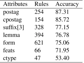
A number of experiments were run to determine the best attribute combinations for each language. Table 4 gives a set of results for single attributes in Spanish. These results are based on 10,000 training instances and all experiments use context=1. Postag was naturally the most informative single attribute on all languages tested, however the second best or the best combination varied between languages. Suffix[3] indicates all suffixes up to three characters in length. TheFEATS column was split into its
con-stituent features each of which was treated as a bi-nary attribute.
Attributes Rules Accuracy postag 254 87.31 cpostag 154 85.72 suffix[3] 328 77.15 lemma 394 76.78 form 621 75.06 feats 66 71.95 ctype 47 53.40
Table 4: Attributes vs. accuracy in Spanish.
There are various reasons for performing at-tribute selection. Intuitively, including more infor-mation should be good, so why not use all the at-tributes? First, not every machine learning algo-rithm is equally tolerant of redundant or irrelevant attributes. Naive Bayes gets 81.54% and C4.5 gets 86.32% on the Spanish data with the single postag attribute using context=1. One reason I chose GPA was its relative tolerance to redundant or irrelevant attributes. However, no matter how robust the algo-rithm, the lack of sufficient training data will pose a problem: it becomes difficult to distinguish informa-tive attributes from non-informainforma-tive ones if the data is sparse. About half of the languages in this study had less than 100,000 words of training data. Fi-nally, studying the contribution of each attribute type in each language is an interesting research topic in its own right. The next section will present the best attribute combinations and the resulting accuracy for each language.
3.2 Results
Language Attributes Accuracy
Arabic ALL 76.87
[image:3.612.325.528.373.550.2]Chinese postag, cpostag 84.51 Czech postag, lemma 79.25 Danish postag, form 86.96 Dutch postag, feats 85.36 German postag, form 87.97 Japanese postag, suffix[2] 95.56 Portuguese postag, lemma 90.18 Slovene ALL 85.19 Spanish postag, lemma 89.01 Swedish postag, form 83.20 Turkish ALL 85.27
Table 5: Adjacent word link accuracy.
[image:3.612.113.261.575.686.2]could not be tested and only the first 100,000 train-ing instances were used. Exceptions are indicated with “ALL”, where all attributes were used in the model – these are cases where using all the attributes outperformed other subsets tried.
For most languages, the adjacent word link accu-racy is in the 85-90% range. The outliers are Ara-bic and Czech at the lower end, and Japanese at the higher end. It is difficult to pinpoint the exact rea-sons: Japanese has the smallest set of link types, and Arabic has the greatest percentage of adjacent word links. Some of the differences between the languages come from linguistic origins, but many are due to the idiosyncrasies of our particular data set: number of parts of speech, types of links, qual-ity of the treebank, amount of data are all arbitrary factors that effect the results. One observation is that the ranking of the languages in Table 5 according to performance is close to the ranking of the best re-sults in the CoNLL shared task – the task of linking adjacent words via machine learning seems to be a good indicator of the difficulty of the full parsing problem.
4 Long Distance Dependencies
Roughly half of the dependency links are between non-adjacent words in a sentence. To illustrate how we can extend the previous section’s approach to long distance links, consider the phrase “kick the red ball”. The adjacent word linker can only find thered-balllink even if it is 100% accurate. How-ever once that link has been correctly identified, we can drop the modifier “red” and do a second pass with the words “kick the ball”. This will identify the linkthe-ball, and dropping the modifier again leaves us with “kick ball”. Thus, doing three passes over this word sequence will bring all linked words into contact and allow us to use our adjacent word linker. Table 6 gives the percentage of the links discovered in each pass by a perfect model in Spanish.
Pass: 1 2 3 4 5
Link%: 51.09 23.56 10.45 5.99 3.65
Table 6: Spanish links discovered in multiple passes.
We need to elaborate a bit on the operation of “dropping the modifiers” that lead from one pass to
the next. After the discovery of the red-ball link in the above example, it is true that “red” can no longer link with any other words to the right (it can-not cross its own head), but it can certainly link with the words to the left. To be safe, in the next pass we should consider boththe-redandthe-ballas can-didate links. In the actual implementation, given a partial linkage, all “potentially adjacent” word pairs that do not create cycles or link crossings were con-sidered as candidate pairs for the next pass.
There are significant differences between the first pass and the second pass. Some word pairs will rarely be seen in contact during the first pass (e.g. “kick ball”). Maybe more importantly, we will have additional “syntactic” context during the sec-ond pass, i.e. information about the modifiers dis-covered in the first pass. All this argues for building a separate model for the second pass, and maybe for further passes as well.
In the actual implementation, models for three passes were built for each language. To create the training data for the n’th pass, all the links that can be discovered with (n-1) passes are taken as given, and all word pairs that are “potentially adjacent” given this partial linkage are used as training in-stances. To describe each training instance, I used the attributes of the two candidate words, their sur-face neighbors (i.e. the words they are adjacent to in the actual sentence), and their syntactic neighbors (i.e. the words they have linked with so far).
To parse a sentence the three passes were run se-quentially, with the whole sequence repeated twice2.
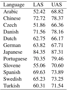
Each pass adds new links to the existing partial link-age, but does not remove any existing links. Table 7 gives the labeled and unlabeled attachment score for the test set of each language using this scheme.
5 Conclusion
I used standard machine learning techniques to in-vestigate the lower bound accuracy and the impact of various attributes on the subproblem of identify-ing dependency links between adjacent words. The technique was then extended to identify long dis-tance dependencies and used as a parser. The model gives average results for Turkish and Japanese but
Language LAS UAS Arabic 52.42 68.82 Chinese 72.72 78.37 Czech 51.86 66.36 Danish 71.56 78.16 Dutch 62.75 66.17 German 63.82 67.71 Japanese 84.35 87.31 Portuguese 70.35 79.46 Slovene 55.06 70.60 Spanish 69.63 73.89 Swedish 65.23 73.25 Turkish 60.31 71.54
Table 7: Labeled and unlabeled attachment scores.
generally performs below average. The lack of a specialized parsing algorithm taking into account sentence wide constraints and the lack of a prob-abilistic component in the model are probably to blame. Nevertheless, the particular decomposition of the problem and the simplicity of the resulting models provide some insight into the difficulties as-sociated with individual languages.
References
A. Abeill´e, editor. 2003. Treebanks: Building and Us-ing Parsed Corpora, volume 20 ofText, Speech and Language Technology. Kluwer Academic Publishers, Dordrecht.
S. Afonso, E. Bick, R. Haber, and D. Santos. 2002. “Flo-resta sint´a(c)tica”: a treebank for Portuguese. InProc. of the Third Intern. Conf. on Language Resources and Evaluation (LREC), pages 1698–1703.
N. B. Atalay, K. Oflazer, and B. Say. 2003. The annota-tion process in the Turkish treebank. InProc. of the 4th Intern. Workshop on Linguistically Interpreteted Cor-pora (LINC).
A. B¨ohmov´a, J. Hajiˇc, E. Hajiˇcov´a, and B. Hladk´a. 2003. The PDT: a 3-level annotation scenario. In Abeill´e (Abeill´e, 2003), chapter 7.
S. Brants, S. Dipper, S. Hansen, W. Lezius, and G. Smith. 2002. The TIGER treebank. In Proc. of the First Workshop on Treebanks and Linguistic Theories (TLT).
S. Buchholz, E. Marsi, A. Dubey, and Y. Krymolowski. 2006. CoNLL-X shared task on multilingual depen-dency parsing. In Proc. of the Tenth Conf. on
Com-putational Natural Language Learning (CoNLL-X). SIGNLL.
K. Chen, C. Luo, M. Chang, F. Chen, C. Chen, C. Huang, and Z. Gao. 2003. Sinica treebank: Design criteria, representational issues and implementation. In Abeill´e (Abeill´e, 2003), chapter 13, pages 231–248.
M. Civit Torruella and MaA. Mart´ı Anton´ın. 2002. De-sign principles for a Spanish treebank. InProc. of the First Workshop on Treebanks and Linguistic Theories (TLT).
S. Dˇzeroski, T. Erjavec, N. Ledinek, P. Pajas, Z. ˇZabokrtsky, and A. ˇZele. 2006. Towards a Slovene dependency treebank. In Proc. of the Fifth Intern. Conf. on Language Resources and Evaluation (LREC).
J. Hajiˇc, O. Smrˇz, P. Zem´anek, J. ˇSnaidauf, and E. Beˇska. 2004. Prague Arabic dependency treebank: Develop-ment in data and tools. InProc. of the NEMLAR In-tern. Conf. on Arabic Language Resources and Tools, pages 110–117.
Y. Kawata and J. Bartels. 2000. Stylebook for the Japanese treebank in VERBMOBIL. Verbmobil-Report 240, Seminar f¨ur Sprachwissenschaft, Univer-sit¨at T¨ubingen.
M. T. Kromann. 2003. The Danish dependency treebank and the underlying linguistic theory. InProc. of the Second Workshop on Treebanks and Linguistic Theo-ries (TLT).
Volkan Kurt. 2005. Protein structure prediction using decision lists. Master’s thesis, Koc¸ University.
J. Nilsson, J. Hall, and J. Nivre. 2005. MAMBA meets TIGER: Reconstructing a Swedish treebank from an-tiquity. InProc. of the NODALIDA Special Session on Treebanks.
K. Oflazer, B. Say, D. Zeynep Hakkani-T¨ur, and G. T¨ur. 2003. Building a Turkish treebank. In Abeill´e (Abeill´e, 2003), chapter 15.
Ronald L. Rivest. 1987. Learning decision lists. Ma-chine Learning, 2:229–246.
L. van der Beek, G. Bouma, R. Malouf, and G. van No-ord. 2002. The Alpino dependency treebank. In Com-putational Linguistics in the Netherlands (CLIN).