Abstract— In this paper, a Neuro-Predictive (NP) controller is
designed and implemented on a highly non-linear system, a model helicopter in a constrained situation. It is observed that the closed loop system with the NP controller has a significant overshoot and a long settling time in comparison to the same system with an existing fuzzy controller. In order to improve the undesired system performance, a Sugeno-type fuzzy compensator, having only two rules, is added to the control loop to adjust control input. The newly designed Neuro-Predictive control with Fuzzy Compensator (NPFC) improves the system performance in both overshoot and settling time. Furthermore, it is shown that the NPFC controlled system is robust to disturbance and parameter changes.
Index Terms—Neuro-Predictive, Fuzzy Control, Model
Helicopter, Overshoot.
I. INTRODUCTION
Predictive control, as a method of using predicted outputs to determine control inputs, was initially introduced by classical Model Predictive Controllers (MPCs) [1]. It is obvious that for “prediction”, a “model” is needed in the classical MPCs. Quite often linear state space models are used. Such models can predict the behavior of many processes satisfactorily [2]. In some cases, Artificial Neural Network (ANN) can use linear models with limited validity areas for non-linear systems; such models can also be used in the classical predictive control [3]. But nonlinear models are usually needed in order to predict the behavior of nonlinear systems. Soloway and Haley used nonlinear artificial neural networks as a model for predictive control purposes [4]. Using nonlinear models, the classical MPC method to derive control input is not applicable any more. In order to compute the control input in the presence of nonlinear ANN models, nonlinear optimization methods are often used [5,6,7], although an additional ANN can also perform this task [8]. Neuro-predictive controllers have been implemented in a variety of applications such as control of food or chemical processes and control of air/fuel ratio of engines [9,
Manuscript received March 5, 2007.
Two authors are both with the School of Mechanical Engineering, The University of Adelaide, South Australia, (corresponding author phone number: +61 8 8303 3156 and e-mail: morteza@ mecheng.adelaide.edu.au, [email protected].).
10, 11]. This method has also been used to control a hybrid water and power supply [12] and a 6-DOF robot [13]. In medical engineering, neuro-predictive controllers are used to control insulin pump of diabetic patients [14]. In this research, neuro-predictive approach is used to control a model helicopter’s yaw movement. A fuzzy inference system is also designed as a compensator to improve the efficiency of neuro-predictive controller.
II. RELATED CONTROL METHODS
The designed hybrid controller includes three main parts; an artificial neural network to predict the behaviour of system, a “nonlinear optimization method” to minimize the performance function, and a “fuzzy inference system” to improve the efficiency.
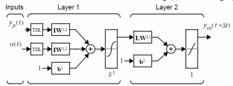
[image:1.595.313.541.492.576.2]Inasmuch as the controlled system is dynamic in nature, the ANN should be recurrent. The inputs of the ANN are the inputs and outputs of system at a specific time (
t
) and at the instants prior to that time. The output of ANN is the output of system at the time just after the specific time, i.e., (t
+
∆
t
), where∆
t
is the minimum time interval of data recording (shown in Fig.1).Figure 1: Scheme of an ANN usable in a neuro-predictive control
A neural network was trained off-line using recorded data before operation; besides, it is trained on-line during operation. A perceptron structure with two layers of connections is used in this study. After training, for the first estimation, the inputs of the ANN are the tentative control input of system (u′), previous control inputs of system (u(k−i) when i≥1), current and previous actual outputs of systems (y(k−i) when i≥0). The output of the ANN is the first predicted value of the output,
) 1 (k+
ys . To estimate ys(k+i), when i>1, the previously estimated values of
y
sare used as previous output values of the system which are originally estimated based upon the actualDesign of an Intelligent Controller for a Model
Helicopter Using Neuro-Predictive Method with
Fuzzy Compensation
outputs of the system, the actual inputs and tentative control inputs of the system.
Predicted outputs of the ANN can be used to calculate the performance function. In the discrete domain, the performance function is defined as below:
, )] 1 ( ) ( [ ] ) ( [ )
( 2 2
1 − − ′ + − + =
∑
= k u k u y i k y k J d N is ρ (1)
where,ysand ydare the estimated and desired outputs of the system respectively, and u′and uare the tentative and actual control inputs, respectively. Additionally,
ρ
is a factor defining the importance of constancy of the control input. In the right-hand side terms of (1) (arguments of Jfunction) u′ is the only independent variable that is not influenced by the current and previous situation of the system. This variable can be selected arbitrarily and can affect other variables and the performance, whereas other terms of the right-hand side of the equation (arguments of J) are thoroughly dependent on the current situation of the system, therefore, their values can not be adjustable. In other words, for control purpose, it can be assumed that:). (u J
J= ′ (2) Now,
u′
should be so determined thatJ
has its minimal value. To do this, the Taylor’s series of the performance function can be written as:), ( ) ( ) ( ) ( u u u J u J u u
J ∆ ′
′ ∂ ′ ∂ + ′ ≅ ′ ∆ +
′ (3) after derivation of (4), it becomes:
). ( ) ( ) ( ) ( 2 2 u u u J u u J u u u J ′ ∆ ′ ∂ ′ ∂ + ′ ∂ ′ ∂ ≅ ′ ∂ ′ ∆ + ′ ∂ (4) In order to minimizeJ(u′+∆u′), its derivative is set to zero. Consequently: . ) ( ] ) ( [ 1 2 2 u u J u u J u ′ ∂ ′ ∂ ′ ∂ ′ ∂ − ≅ ′
∆ − (5)
The right-hand side of (5) is called Newton’s direction [15]. In this method,
g
k, a performance function gradient is defined as:; ) 1 ( ) ( ) 1 ( ) ( ) ( − − ′ − − = = ′ ∂ ′ ∂ k u k u k J k J g u u J
k (6)
moreover, Gk is defined as: . ) 1 ( ) ( ] ) ( [ 1 1 2 2 − − − − − ′ = = ′ ∂ ′ ∂ k k k g g k u k u G u u J (7) To modify control input, following relation can be used:
, k k old new u G g
u
u′= ′ − ′ =−
∆ (8) but, in practice, an adjustable coefficient is used for Gkgkto obtain a quicker convergence:
. k k old
new u Gg
u
u′= ′ − ′ =−η
∆ (9) Using (9), it is obtained that:
), (
)
(unew J uold Gkgk
J ′ = ′ −η (10) Equation (10) can be rewritten as:
. k k old G g
u J of
Argument = ′ −η (11)
Both uold′ and Gkgk are known in this stage, then, while changingη, Argumentof J moves along a line. There is an optimum point on this line that minimizes J . Such an optimization problem is classified as a linear search. The backtracking method, introduced by Dennis and Schnabel [16], is selected for linear search. The modified u′(
u′
new) is used as the new control input.Beside neural modeling and selecting optimization (predictive) algorithm, a simple Sugeno-type fuzzy inference system is designed to make the response of neuro-predictive controller decay quickly when the error is sufficiently low.
III. MECHANICAL MODELING
The model helicopter used in this research is a highly nonlinear two input-two output system. The helicopter has two degrees of freedom, the first possible motion is the rotation of the helicopter body with respect to the horizontal axis (which changes the pitch angle) and the second is rotation around the vertical axis (which change the yaw angle). The helicopter can rotate from −170 to 170 in the yaw angle, and from −60to
60 in the pitch angle. System inputs are voltages of main and rear rotors, and the yaw and pitch angles are considered as its outputs.
Figure 2: A scheme of model helicopter
A mechanical modeling was obtained using Newton and Euler laws. After modeling, the following differential equations are obtained [17]:
The variables and indices are listed at nomenclature. In (5~10) the torques can be substituted by their equal expressions obtained from kinetics of the system.
In this research, a special situation is studied. In this situation, the motion is so constrained that the vertical motion is impossible; moreover, the input voltage of main rotor (UR) is set to “zero”. As a result, the only input of the system is the input voltage of rear rotor(US). Also, the yaw angle (the angle in horizontal plane) is considered as the unique output. In this situation, only (16) and (17) can represent the behavior of system. Since there is no change in the pitch angle, gyroscopic torque does not exist; furthermore, the main rotor does not generate any torque. Consequently, (17) is simplified as below:
), (
1
, ,
RearRotorS frictionS V
T T
I dt d
− =
ψ
ω
(18) where:
, )
( 2
,
RearRotorS rSkFSsign S S
T = ω ω (19) .
,S µVωψ
friction c
T = (20) The equations defining the behavior of this first order system can be written as:
, ψ
ω
ψɺ= (16) ),
) ( (
1 2
ψ µ
ψ ω ω ω
ω S FS S S V
V
c sign
k r
I −
=
ɺ
(21) whereωψis the angular velocity of helicopter body in the yaw direction and ωS is the angular velocity of the rear rotor blades that is a nonlinear function of the input voltage of rear rotor.
IV. DESIGN OF HYBRID CONTROLLER
A. Neural Network Model
A three layer recurrent perceptron is used to model the system. The numbers of neurons in the input and hidden layers are 6 and 7 regardless of biases. The value of each bias is 1. The input and output layers have linear activation functions with slope of one, whereas, the hidden layer has sigmoid activation function, that is, the output of ith neuron of the hidden layer is:
), tanh(
7
1
∑
= =
j j ij
i w y
o (22) where
w
ij is the weight of connections between ith neuron of the hidden layer and jth neuron of the input layer whose output isj
y
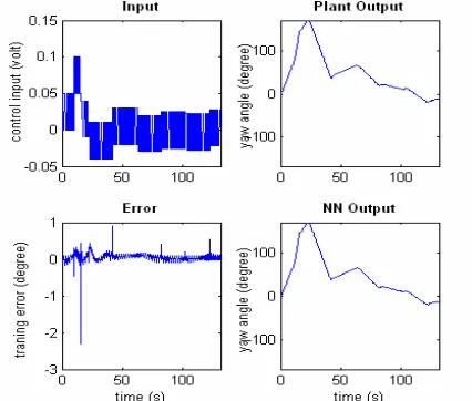
, and 7 (at the top of sigma symbol) is the number of neurons in the input layer in addition to its bias. In this research, Levenberg-Marquardt algorithm is applied for batch back-propagation training. A scheme of neural network together with the input and output data during training is shown in Fig. 3. A set of 1300 input-output recorded data of system was used for training. In order to obtain such a data set, pulse signals were sent to the system with a time interval of 1 second for 130 seconds and the output value was recorded at any time. Testing data was obtained with sending a sinusoidal signal to the system as the input (input is the voltage of the rear rotor of the helicopter). The training was completed only with 8 iterations.Figure 3: Neural network structure and input-output data in training stage
[image:3.595.322.525.253.435.2]The performance function of training is the sum of squared errors, and the data were normalized before training. Figures 4 and 5 both illustrate the success of training.
Figure 4: Verification information of ANN regarding testing area
Figure 5: Verification information of ANN regarding training area
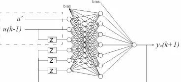
After successful training, the neural network was used to predict the future outputs of the system. In this stage, dissimilar to training stage, the inputs and outputs were not recorded data. For the first estimation, the neural network inputs and outputs are shown in Fig.6.
[image:3.595.319.532.466.647.2]replaced byys(k+i) (where i>1); moreover, some of the inputs of the ANN shown in a dashed rectangle in Fig.7, change values when ys(k+i) (where i>1)is estimated. For i=2, or to estimate ys(k+2), the inputs of the ANN located in the dashed rectangle of Fig.6, are shown in Fig.7.
[image:4.595.77.262.156.239.2]Figure 6: Neural network structure and input-output data in the first estimating (predicting) stage
Fig.8 shows the same inputs for
i
≥
3
.Figure 7: dashed area of Fig.6 for i=2
Figure 8: dashed area of Fig.6 for i>2
B. Predictive Control
In order to explain the details of predictive control, (1) should be re-noticed:
. )] 1 ( ) ( [ ] ) ( [ )
( 2 2
1
− − ′ + − +
=
∑
=
k u k u y i k y k
J d
N
i
s ρ
The purpose of predictive control is to define tentative control input
u′
so that Jis minimized. Using the ANN, designed and trained in previous section, predicted output values can be available. To obtain predicted output values, at each instant, the ANN should be used Ntimes as shown in (1). The estimated (predicted) output value of any stage of prediction is applied as one of the inputs for the next prediction stage. In this research7
=
N has been used. Let’s consider seven sequential identical neural networks that the outputs of any of them (except the last one) provide one of the inputs of the next ANN. Such a neural model, namely “Neural Predictive Model” obtains the estimated (predicted) output values of system (y(k+i), i=1~7) using the previous and current values of the output of system(y), the previous values of control input (u) and the tentative control input (u′) . As a result, when ρ=1or2 , the value of performance function (J) can be calculated as shown in Fig.9. In order to explain the total process of predictive control, a general model is considered as the sum of neural predictive model and
J
function. The output of this general model is the value ofJ
(
k
)
. Additionally, as previously stated, the nonlinear optimization function which derives the tentative control input is a combination of (6), (7), (9) and the linear search. Fig.10 shows the neuro-predictive control algorithm. [image:4.595.47.240.272.385.2]Figure 9: The process of calculation of the performance function
Figure 10: neuro-predictive controller
For the first steps, J(−1) and J(−2) should be determined using previous recorded values.
C. Fuzzy Compensator
After implementation of neuro-predictive controller, it was observed that it reached the desired point more quickly than existing fuzzy controller, but a serious problem was also observed. The system under neuro-predictive control has a considerable overshoot and a long settling time. In order to solve this problem, a fuzzy compensator is added to the controller. The input of this fuzzy inference system is the absolute value of error and its output is a coefficient multiplying by u′ (the tentative control input, derived from the neuro-predictive algorithm) to achieve a modified control input. This fuzzy compensator is a Sugeno-type FIS with only two rules:
if absolute error is A then correction coefficient=2;
if absolute error is any value then correction coefficient=0;
where A is a Gaussian membership function whose membership grade can be calculated as below:
] ) 5
20 (
2 1
exp[− − 2
= absoluteerror
mg . (23)
A scheme of this fuzzy inference system is shown in Fig.11.
Figure 11: fuzzy compensator scheme
[image:4.595.305.544.531.676.2]V. SIMULATION RESULTS
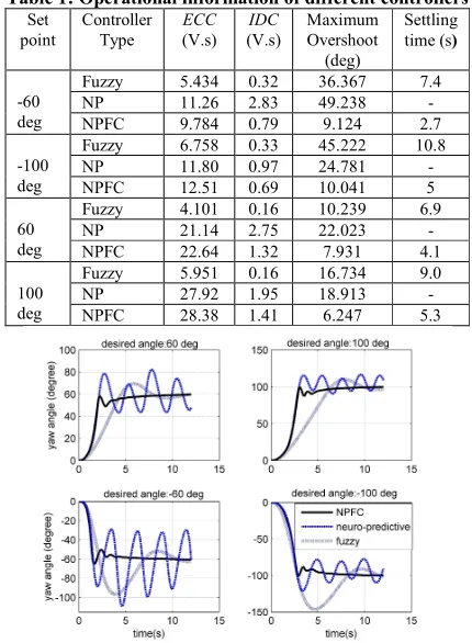
[image:5.595.60.275.191.484.2]The responses of the closed loop system for the three different controller are shown in Fig.12 for four set-points and three controllers. In other words, the helicopter was rotated form stationary situation to some different desired values of yaw angle by the rear rotor, while the rear rotor was controlled by an existing “fuzzy controller”, “neuro-predictive controller” or “NPFC”.
Table 1: Operational information of different controllers
Set point
Controller Type
ECC
(V.s)
IDC
(V.s)
Maximum Overshoot
(deg)
Settling time (s)
Fuzzy 5.434 0.32 36.367 7.4
NP 11.26 2.83 49.238 -
-60
deg NPFC 9.784 0.79 9.124 2.7
Fuzzy 6.758 0.33 45.222 10.8
NP 11.80 0.97 24.781 -
-100
deg NPFC 12.51 0.69 10.041 5
Fuzzy 4.101 0.16 10.239 6.9
NP 21.14 2.75 22.023 -
60
deg NPFC 22.64 1.32 7.931 4.1
Fuzzy 5.951 0.16 16.734 9.0
NP 27.92 1.95 18.913 -
100
deg NPFC 28.38 1.41 6.247 5.3
Figure 12: Responses of different controllers & setpoints
An energy consumption criterion (ECC) is also defined to represent the total energy consumption of the closed loop system during operation, and it can be calculated as:
, ) (
0
dt t u ECC
T
∫
= (24)
where
T
is the final time for calculation and u(t)is the input voltage of the helicopter’s rear rotor or control input. Since neuro-predictive controllers are essentially designed to reduce the deviation of inputs rather than the absolute value of inputs. Another criterion namely, input deviation criterion IDC is defined as:, ) ( )
(t ut dt u
IDC
T
∫
− −=
τ
[image:5.595.330.517.581.728.2]τ (25) where
τ
is the sampling time of the system. Table 1 includes these two criteria for all plots shown in Fig.12. This table also shows information of the maximum overshoot of the experiments. Furthermore, the settling time needed for the yaw angle to settle within 5 degrees of the desired value, is shown in Table 1 as well.It is clearly observed that the proposed NPFC controller performs better in terms of the overshoot and settling time in comparison to the existing fuzzy controller which is considered as a satisfactory controller for this type of high inertia systems. From the simulations, it can be seen that the control input generated by NPFC controller does not exceed the permitted range for the input voltage although it consumes more energy.
VI. ROBUSTNESS ANALYSIS
In this section, the designed controller (NPFC) is experimentally evaluated regarding the parameter or disturbance robustness. At the first step, a NPFC controller with ρ=2 is designed. In order to elaborate disturbance robustness, the helicopter was exposed to a sudden impact causing 30 rotations in the direction or against the direction of
rotation. The disturbances (impacts) are exerted around the sixth second during system’s operation as shown in Fig. 13. At the same moment the error was about 2 and converged to zero.
The desired yaw angles were 80 and −80 . The assumed
impacts were considerably severer than those impacts may be encountered in reality. The controlled system passed these experiments successfully. Fig.13 shows the response of the NPFC controlled system under the mentioned disturbances.
In order to analyze the parameter robustness of the system, (16) and (21) defining systems’ dynamic can be re-written as:
, ψ
ω
ψɺ= ).
) ( (
1 2
ψ µ
ψ ω ω ω
ω S FS S S V
V
c sign
k r
I −
=
ɺ There are four parameters in these equations: the moment of inertia IVfor the helicopter body around its vertical axis, the distance of the rear rotor rSfrom the joint of the helicopter body with its basis (shown in Fig.3), the rear rotor blade constant kFS
and the friction coefficient for rotation around vertical axis V
c
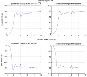
µ . Among these parameters, IV and rS are geometrical constants. As to the operation environment of the model helicopter,kFS is also assumed to be a constant. Therefore, the only variant parameter of system is cµVwhose original value for properly lubricated joint is 0.0095.Dust or lack of fabrication may cause this parameter increased. Figs.14 and 15 show the effect of a sudden increase of this parameter by 300% during operation. The increase of
V
[image:6.595.76.257.159.319.2]cµ occurred at the fourth and sixth second time marks. The NPFC controlled system passed the tests satisfactorily.
Figure 14:The behavior of NPFC controlled system with sudden parameter change
Two main reasons can be attributed to the robustness of the NPFC controller;
1) The output of fuzzy compensator’s output (and consequently controller’s input) increases considerably as soon as the absolute error increases. 2) On-line training makes the neural network model
adaptive to changes in parameters.
VII. CONCLUSION
In this paper, neuro-predictive controllers are studied and implemented on a system with non-linear and non-symmetric dynamics. Although pure neuro-predictive controllers do not work well for this system, but NP controllers, combined with a fuzzy compensator, shows a satisfactory response in comparison to the existing fuzzy controllers. In the NPFC the control input is adjusted through multiplying by a small positive number generated by fuzzy inference system. The fuzzy compensator is designed so that as the error is small, the output converges to zero. It is indicated that the designed controllers improve the control performance of the closed loop system. Moreover, the disturbance and parameter robustness of the system has been improved as well.
REFERENCES
[1] E. Fernández Camacho, C. Bordons, “Model Predictive Control” Springer, 2004
[2] A. Ghafari, M. Nikkhah Bahrami and M. Mohammadzaheri, "Linear Modeling of Nonlinear Systems Using Artificial Neural Networks Based on I/O Data and Its Application in Power Plant Boiler Modeling (in Persian)", Journal of Engineering Faculty of University of Tehran/ Mechanics and Metallurgy, 39 (1) (2005) 53-60.
[3] R.K. Al Seyab, Y. Cao ,”Nonlinear model predictive control for the ALSTOM gasifier” Journal of Process Control Vol.16 (2006),pp. 795–808.
[4] Soloway, D. and P.J. Haley, “Neural Generalized Predictive Control,” Proceedings of the 1996 IEEE International Symposium on Intelligent Control, 1996, pp. 277-281.
[5] Razi, M. Farrokhi, M. Saeidi, M.H. Khorasani, A.R.F.Neuro-Predictive Control for Automotive Air Conditioning System, International Conference on Engineering of Intelligent Systems, 2006 IEEE, 22-23 April 2006 pp.: 1 – 6.
[6] Yun Zhang,“The research on the GA-based neuro-predictive control strategy for electric discharge machining process”, International Conference on Machine Learning and Cybernetics”, 26-29 Aug. 2004 Volume: 2,pp. 1065 - 1069
[7] Alexander G. Parlos, , Sanjay Parthasarathy, and Amir F. Atiya, “Neuro-Predictive Process Control Using On-Line Controller Adaptation”, IEEE Transactions on Control system Technology Vol.9, No. 5, September 2001
[8] Jean-Pierre Vila, V'erene Wagner, “Predictive neuro-control of uncertain systems: design and use of a neuro-optimizer”, Automatica Vol. 39 (2003) pp. 767 – 777.
[9] M. Morari, C.E. Garcia, J.H. Lee, D.M. Prett; “Model Predictive Control”; Prentice Hall, 1994.
[10] Bernt M. Akesson, Hannu T. Toivonen, “A neural network model predictive controller”, Journal of Process Control,Volume 16, Issue 9,October 2006,pp.937-946.
[11] S.W. Wang, D.L. Yu, J.B. Gomm, G.F. Page, S.S. Douglas, “Adaptive neural network model based predictive control for air–fuel ratio of SI engines”, Engineering Applications of Artificial Intelligence vol.19 (2006) pp.189–200
[12] Ali Al-Alawi, Saleh M Al-Alawi, Syed M Islam, “Predictive control of an integrated PV-diesel water and power supply system using an artificial neural network” , Renewable Energy Volume 32, Issue 8, July 2007, pp. 1426-1439.
[13] Rasit Koker,” Design and performance of an intelligent predictive controller for a six-degree-of-freedom robot using the Elman network”,
Information Sciences 176 (2006) pp. 1781–1799
[14] Gaston Schlotthauer, Lucas G. Gamero, Maria E. Torres, Guido A. Nicolini “Modeling, identification and nonlinear model predictive control of type I diabetic patient” Medical Engineering & Physics vol. 28 (2005) pp.240–250
[15] J. R. Jang, C. Sun, E. Mizutani. “Neuro-Fuzzy and Soft Computing”, Prentice-Hall Inc.1997.
[16] Jr., J.E. Dennis and Robert B. Schnabel, “Handbooks in Operations Research and Management Science, Volume 1, Optimization, Chapter I A view of unconstrained optimization, pp. 1-72.