Parallel Implementation of Hybrid Direct-Iterative Algorithm for Multibody Dynamics via Krylov Subspace Methods on IBM 1350 Cluster

Abstract—In this paper, a new hybrid direct-iterative algorithm for multibody dynamics is discussed. The implementation of the algorithm on IBM 1350 cluster is then presented. Some Krylov subspace methods available in Aztec library are utilized to solve constraint equations for real parallel implementation using MPI. The parallel simulation results are further compared with the results produced from different iterative solvers. Integration between the new algorithm and Aztec will make the algorithm accommodate various multibody systems easily while keeping its high simulation speed.

Keywords — hybrid direct-iterative algorithm, Krylov subspace method, multibody system (MBS), parallel computing

I. INTRODUCTION

With the development of various parallel computer systems, the techniques provided by these systems and the concurrent nature of MBS have been receiving increasing attention. A few parallel algorithms for computer simulation of dynamical behaviors of MBS have been put forward by individuals whose interests may lie in various fields since the first parallel MBS algorithm developed by Kassahara, Fujii, and Iwata in 1987 [1]. In 1988, Bae, Kuhl and Haug [2] applied the recursive algorithms developed by them to a shared memory multiprocessor system to realize parallel computing of MBS. Lee [3] presented a global _O(_n3)_{algorithm from its inception}

to develop the equations of motion in such a way as to allow the exploitation of the concurrent processing to the maximum degree on a multiple instruction multiple data (MIMD) machines. Based on his previous work [4] in 1990, Anderson [5] demonstrated that significantly greater parallelism could be realized with a modified form of theO(n)algorithm. Fijany and Bejczy [6] showed that the more traditional

)

(

_n

3

O

methods provide the highest degree of parallelism in 1993. Sharf and D’Eleuterio presented a new parallel solution procedure for dynamic simulation of multibody chains by solving joint constraint forces via various iterative parallel methods [7]. Based on parallel strategies for constraint equations in [7], Fijany, Sharf, and D’Eleuterio [8] implemented Constraint-Force algorithm (CF) on parallel computing system with

O

(

N

)

processors for solving both equations of motion and constraint equations. Anderson and Duan presented a new direct-iterative algorithm (HDIA) for multibody chain systems [9] and implemented it on IBM SP2 and SGI ONYX [10]. In their work, MBS is constructed

S. Z. Duan is a faculty member with the South Dakota State University, College of Engineering, Mechanical Engineering Department, Brookings, SD 57007 USA (the corresponding author: phone: 605-688-5930; fax: 605-688 -5878; e-mail: shawn.duan@ sdstate.edu).

Y. Patel is a graduate student with the South Dakota State University, College of Engineering, Mechanical Engineering Department, Brookings, SD 57007 USA

so that largely independent multibody subchain systems are formed. They specifically applied the HDIA to a pure chain system and used a 16 body chain for parallel implementation of their HDIA approach with various joint cutting on IBM SP2 and SGI ONYX with MPI-supported environment. The work presented in this paper is an integration of HDIA with Krylov methods used in Aztec iterative solvers [11] to extend computational power and application abilities of HDIA.

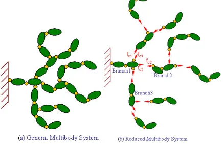
II. HYBRID ITERATIVE-DIRECT ALGORITHM (HDIA) In HDIA approach, the MBS model is constructed through the separation of certain key system interbody joints so that largely independent multibody subchain systems are formed. These subchains in turn interact with one another through associated unknown constraint loads fc at those separated

[image:1.612.321.540.346.487.2]

joints as shown in figure 1. The added parallelism is obtained through this separation and the explicit determination of fcby

Figure 1: A MBS & Its Associated Subchains parallel iterative methods at a coarse grain level. Each branch is assigned to a processor of a parallel computing system for parallel simulation. An efficient sequential O(n) procedure is carried out to form and solve equations of motion within each processor, while parallel strategies are used to form and solve constraint equation between the processors concurrently. The O(n) method is embedded with direct method for formation and solution of equations of motion so that once the equations of motion is formed they have been solved. The parallel strategies take advantages provided by iterative method. Thus HDIA takes a combination of direct and iterative approaches. In HDIA, the equations of motion and constraint equation have the following form, respectively

)

,

,

,

(

)

,

(

t

q

u

R

t

q

u

f

_c

M

⋅

=

)

,

,

,

(

t

q

u

f

_c

RHS

u

=

(1a)

)

,

,

(

)

,

(

t

q

⋅

f

_c

=

Ψ

t

q

u

Γ

(1b)

In equation (1a) and (1b),

M

is the system mass matrix implicitly formed by using the sequential O(n) procedure.

q

Parallel Implementation of Hybrid Direct-Iterative Algorithm for Multibody Dynamics via

Krylov Subspace Methods on IBM 1350 Cluster

are the generalized coordinate column-matrix used to define the configuration of MBS,

u

are generalized speed column- matrix that characterizes the motion of the system, and

u

are the generalized accelerations that are to be determined. The matrix

RHS

is right hand side matrix which contains all of external loads, body loads, constraint forces, and as well as inertia forces and torques associated with centripetal and Coriolis accelerations. Generally, the elements of

RHS

are nonlinear functions of the system state variables and time. The matrix

Γ

is the constraint coefficient matrix and the matrix

Ψ

consists of nonlinear functions of state variables and time. Finally,

f

_c is the unknown constraint force measuring numbers that must exist at separated joints between subchains of the reduced system, which makes the reduced system behave like the original system.

There are five computational tasks associated with forming and solving equation (1a) and (1b) as shown in figure 2. Next HDIA associated with these five computational tasks will be discussed and presented.

Task 1 Forming Equation of Motion (1a)

Task 2 Solving Equation of Motion (1a)

Task 3 Forming Constraint Equation (1b)

Task 4 Solving Constraint Equation (1b)

Task 5 Determining State Variables

& Integration

Pr

ec

ed

en

ce

T

im

e

Low High

Task 1 Forming Equation of Motion (1a)

Task 2 Solving Equation of Motion (1a)

Task 3 Forming Constraint Equation (1b)

Task 4 Solving Constraint Equation (1b)

Task 5 Determining State Variables

& Integration Task 1

Forming Equation of Motion (1a)

Task 1 Forming Equation of Motion (1a)

Task 2 Solving Equation of Motion (1a)

Task 2 Solving Equation of Motion (1a)

Task 3 Forming Constraint Equation (1b)

Task 3 Forming Constraint Equation (1b)

Task 4 Solving Constraint Equation (1b)

Task 4 Solving Constraint Equation (1b)

Task 5 Determining State Variables

& Integration Task 5 Determining State Variables

& Integration

Pr

ec

ed

en

ce

T

im

e

[image:2.612.310.544.126.533.2]

Low High

Figure 2: Precedence and Parallelism between Tasks In the following mathematical representation of the HDIA algorithm, Kane’s equations [12] are taken as axiomatic. The detail derivation of general formulations of the HDIA method is presented in references [9, 13, 14]. A notation convention with key joints Jk of body Bk belonging to subchain i may be

used as shown in figure 3.

k k

J

B

i

r

N

ω

Figure 3: An Example for Notation Convention

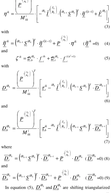
A. Formation and Solution of Equations of Motion In HDIA, generalized accelerations in equations of motion (1a) can be expressed in the form

ik ik ik

u

=

η

+

ζ

(

k

=

1

,

2

,...,

ν

i

)

(2) where scalar quantity

ν

iis degree of freedom (DOF) of

subchain i, scalar quantity

ζ

ikis the generalized acceleration that results from the unknown constraint forces and scalar quantity

η

ik is the generalized acceleration from all other forcing terms. Both of them can be determined using the following recursive formulations

(

)

_⋅

( )

₊

⋅

−

⋅

=

_{k k− k} − k

k k k

B k J i

iB k i T iB iB B J i iB i

kk T

ik

_I

_S

_F

M

P

ˆ

~

ˆ

1

η

1

η

(3) with

(

iB iB

)

T i( )k ik

ik Bk

k J i k

k

S

η

P

η

η

~

=

−1

⋅

~

−1

+

⋅

₍

η

~

ik_{=0) (4)}

and

) 1 (

6 _{+ ⋅} +

⋅

= k k i i

c iB t i c iB b

ik _{f f} υ

ζ

(5)

with

(

)

⋅

⋅

−

⋅

=

ˆ

_{k k−1 k} k−1

k k k

B k J i

k iB

t T iB iB B J i iB ik t i

kk T

iB

t

I

S

D

M

P

D

τ

(6) and

(

)

⋅

⋅

−

⋅

=

ˆ

_{k k−1 k} k−1

k k k

B k J i

k iB

b T iB iB B J i iB ik b i

kk T

iB

b

I

S

D

M

P

D

τ

(7) where

(

)

Bk k

k J i k k

k

k iB

t iB

t T iB iB iB

t

S

D

P

D

D

=

₋₁

⋅

−1

+

⋅

(

D

iB_t 0=0) (8) and

(

)

Bk k

k J i k k

k

k iB

b iB

b T iB iB iB

b

S

D

P

D

D

=

₋₁

⋅

−1

+

⋅

( iB0

t

D

=0) (9) In equation (5), iBk

t

D

and iBk

b

D

are shifting triangularized and backsubstituted constraint Boolean matrix, while

f

i_c6 and

f

i_c(υi+1) are constraint load components applying to base body and terminal body of subchain i respectively. In formula (3), (6), and (7), k

k

k _B

J i iB

I

ˆ

_∈

_R

6×6_{is the articulated inertia}

matrix of body k of subchain i, and scalar term

M

_kki is the diagonal element of the mass matrix

M

associated with equation (1a). Both of them can be recursively determined by

(

_{iB iB}

)

T B

J i iB iB iB B J i iB B J i

iB _{k k k} k k_{k k k}

k k k k k

S I

T I

I 1 1

1 1

1 ˆ

ˆ + +

+ +

+⋅ ⋅

+

= (10)

⋅

⋅

=

Bk

k J i k k

k k B

k J i

P

I

P

M

B

J i iB T i

kk (11)

subchain i

body k

index

reference frame N joint k

[image:2.612.81.290.314.478.2]

Matrix Bk

k J i

P

is the partial velocity matrix associated with DOF of joint k of subchain i, and matrixiBk

S

iBk+1_{is a linear}

transformation matrix that shifts forces and inertias from the inboard joint of body k to an equivalent force/moment system acting on the inboard joint of body k-1. Matrices

τ

ik_t and

τ

ik_b in equations (6) and (7) are the shift-triangularization matrices that shift constraint measure numbers i6

c

f

and

) 1 ( i+

i c

f

υ from their original acting point on the base body and terminal body to the proximal joint of body k during triangularization of O(n) algorithm.

F

ˆ

iBk

_∈

_R

6×1_{in equation}

(3) is the articulated body force matrix of body k of subchain i, and is determined recursively from

1

1

ˆ

ˆ

₊ +

⋅

+

=

_{k k k} k

k iB iB iB iB

iB

F

T

F

F

(12)

where iBk−1

T

iBk

∈

_R

6×6_{is the triangularization operation}

matrix that recursively triangularizes the equations as they are being formed, and is determined from

(

)

⋅ − ⋅ ⋅ ⋅ = − − T B J i iB i kk iB iB iB

iB Bk

k J i k B k J i k k k k k k

k I P P

M U S

T 1 1

1

(13) Through equations (2) – (13), equations of motion (1a) associated with a MBS is formed and solved at a computing cost of

p

N

n

O

[10], where n is number of DOF of the MBS, and Npis number of processors of a parallel computing

system.

B. Formation of Constraint Equations

Formulation of constraint equation (1b) is carried out by enforcing constraints at separating joints (Nsub-1 joints. Nsub: total number of subchains) through following equations

i i c i i i c ii i c i i i i i f f

f + Γ ⋅ − Γ ⋅ =Ψ

⋅ Γ − + + + + + − − +

− _{( 1)( 1)}

) 1 ( ) 1 ( ) 1 )( 1 ( ) 1 ( ) 1 ( ) 1 ( ) ( ) ( )

( υ υ υ

(i=1, 2,...., Nsub-1) (14) where

[

⋅

⋅⋅

]

⋅

=

Γ

₋ i i iBv b iB b iv i i i

D

D

G

G

1 1 1 1 ) 1 (

)

(

, (15)

[

⋅

⋅⋅

]

⋅

+

=

Γ

i i iBv t iB t iv i ii

D

D

G

G

1 1 1 1

)

(

( ) ( )

[

]

( ) ( )

⋅

⋅⋅

⋅

+ + + + 6 1 1 1 6 1 2 1 1 2 B i b B i b i i

D

D

G

G

, (16)

( )

[

( ) ( )

]

( ) ( )

⋅

⋅⋅

⋅

=

Γ

+ + + + + 6 1 1 1 6 1 2 1 1 2 1

)

(

B i t B i t i i i i

D

D

G

G

, (17)

and ( ) ( )

[

]

⋅

−

=

Ψ

+ + + + 6 ) 1 ( 1 ) 1 ( 6 1 2 1 1 2 i i i i

i

G

G

η

η

[

]

( )

i

(

( ) i

)

i i _iB t B i t i i i iv

i

_G

_O

_A

_A

G

ν ν

ν

η

η

−

⋅

+

⋅

⋅⋅

⋅

+1 +1 6

1 1 1 1 (18) with

Ρ

⋅

=

k k B J i ik ik

L

G

1 1 , (19)

T iB iB k i

ik

L

k

S

k

L

( 1)

(

( 1)

)

1

1

=

⋅

+

+

, (20) and ) 1 ( ) 1 ( 1 +

+

₌

i

i _iv

v

i

_O

L

. (21)

Similarly

+ +

+

₌

_⋅

_Ρ

k k B J i k i k i

_L

G

( 1) ( 1) 2

) 1 (

2

(

k

<

7

)

, (22)

T B i B i k i

ik

L

k

S

k

L

( 1)( 1)

(

( 1) ( 1) ( 1)

)

2

2

=

+ +

⋅

+ + +

(

k

<

6

)

, (23)

and ) 1 ( 6 ) 1 ( 2 +

+

₌

_Ο

_ivi

i

L

. (24)

Equations (14)-(24) are algorithmic formulations of equation (1b) for constraint measure numbers fc associated with entire

subchain system. In equation (14), (i−1)( (i−1)+1)

c

f

υ , i( i+1)

c

f

υ , and (i+1)( (i+1)+1)

c

f

υ are the constraint load measure numbers of the separated joints between subchain i-1 and i, subchain i and i+1, and subchain i+1 and i+2, respectively. Matrices

ik

G

₁ and

G

ik₂ are those portions of the constraint coefficient matrix associated with the outboard joint of terminal body and inboard joint of base body, if a subchain is separated at both ends. These quantities play the role of implicitly shifting the DOF of the entire subchain to the separated joints and project these DOF onto the constraint subspace associated with the separated joints.

Ο

i(vi+1)is the orthogonal complement matrix to the free mode of motion matrix (partial velocity matrix)

k B

k J i

P

. The joint orthogonal complement

Ο

i(vi+1)defines the constraint subspace associated with the separated outboard joint on terminal body of subchain i. Matrices

L

1ikand

ik

L

2

are intermediate quantities that are introduced for convenient expression of recursive relations algorithmically. iBi

t

A

ν _in

equation (18) is the acceleration remainder terms of terminal body of subchain i, which are not explicit in the element of

u

. Quantity ( )i 1B6

t

remainder term matrix associated with all of the terms of the relative acceleration matrix not explicit in

u

s

of imaginary body

_ν

i

+

1

_{relative to the terminal body}

_ν

i_{of subchain i.}

Through equations (14) – (24), constraint equation (1b) associated with the reduced MBS is formed at a computing cost of ₂

p

N

nm

O

[10], where m is number of constraints for

the reduced subchain system.

III. SOLUTION OF CONSTRAINT EQUATION

For the work presented in reference [10], a simple in-house Parallel Preconditioned Conjugate Gradient (PPCG) iterative solver was used to solve constraint equation (1b) in parallel. PPCG methods work very well for solution of a large sparse, symmetric, and positive definite system of linear equations. In reality constraint matrix

Γ

seldom has such nice properties. To extend power and application ability of HDIA approach, other Krylov subspace methods such as Generalized Minimal Residual (GMRES), Biconjugate Gradient (BiCG), and Quasi -Minimal Residual (QMR) may be explored and integrated with HDIA. These nonstationary iterative methods have their advantages for solution of a large-sized sparse linear system. For example, by comparison GMRES performs well for non- symmetric systems and QMR works for non-positive definite systems [15]. Nonstationary iterative solvers in Aztec has been used to integrate with HDIA.

A. Aztec Nonstationary Iterative Method Library There are a few massively parallel iterative solver libraries, such as Aztec, PETsc, ScaLAPACK etc. for solving sparse linear systems. Aztec Library has been chosen to integrate with HDIA for solving constraint equation (1b) in parallel because Aztec has a similar coding environment as the HDIA codes and it is ease of availability.

Aztec is a parallel iterative library for solving linear systems, which is both easy-to-use and efficient. It is written in ANSI-standard C language. The source code of Aztec is available freely from the Sandia National Laboratory website. Aztec has been adopted to a number of parallel machines and platforms: workstation clusters (DEC, SGI, SUN, LINUX, etc.), Cray T3E, Intel TeraFlop, Intel Paragon, IBM SP2, nCUBE2 as well as other parallel platforms. There are a number of Krylov subspace methods such as CG, CGS, BiCGSTAB, GMRES, and TFQMR available in Aztec. These Krylov methods may be used in conjunction with various preconditioners. Point & block Jacobi, Gauss-Seidel, and least-squares polynomials are samples of preconditioners in Aztec [11].

B. Integration between HDIA and Aztec Iterative Solvers Aztec can work with user-supplied matrix-vector product routines or two specific sparse matrix formats (in which case Aztec provides the matrix-vector product) - a point entry modified sparse row (MSR) format or a block-entry variable block row (VBR) format. These two formats have been generalized for parallel implementation and, as such, are referred to as “distributed” yielding DMSR and DVBR references. To invoke Aztec from an external program

through a user-supplied matrix-vector product interface, the following steps are required:

1. Describe the machine (serial/parallel) 2. Initialize the matrix and vector data structures 3. Choose the iterative method, preconditioner and the convergence criteria

4. Initialize the right hand side and initial guess 5. Supply the preconditioner

6. Supply the left hand side implicitly through the matrix-vector product routine

7. Invoke the solver

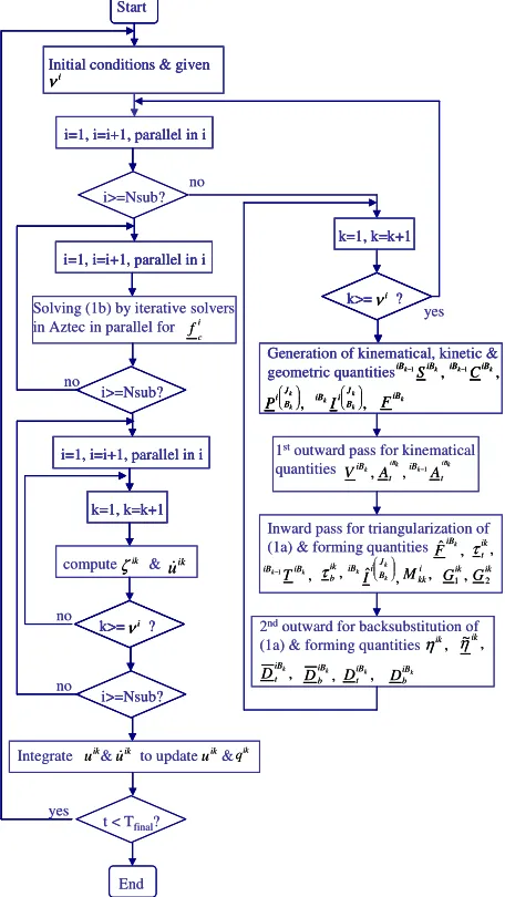
The flow chart in figure 4 shows the integration between HDIA and iterative solvers in Aztec.

Start

Initial conditions & given i

ν

i=1, i=i+1, parallel in i

i=1, i=i+1, parallel in i i>=Nsub?

Solving (1b) by iterative solvers in Aztec in parallel for i

c

f

i=1, i=i+1, parallel in i

k=1, k=k+1

compute &_ζik _uik

k>= ?_νi i>=Nsub?

i>=Nsub?

Integrate & to update & _uik _uik _uik _qik

t < Tfinal?

End

1st_{outward pass for kinematical}

quantities k=1, k=k+1

k>= ?_νi

Generation of kinematical, kinetic & geometric quantities iBk−1_SiBk,iBk−1_CiBk_,

, k k k _B J i iB _{I F}iBk ,

k k B J i

P

, k iB t

A

, k iB

V iBk k

t iB

A

1

−

Inward pass for triangularization of (1a) & forming quantities ˆiBk_,

F

, 1 k k iB iB

T

− _,

1

ik

G

, ˆ k

k k _B J i iB

I i, kk

M

, ik t τ ,

ik b

τ ik

G2

2nd_{outward for backsubstitution of}

(1a) & forming quantities _ηik, ,

k iB t

D

, ~ik η ,

k iB b

D iBk, t

D iBk b

D

no

yes

no

no

no

yes

Start

Initial conditions & given i

ν

Start

Initial conditions & given i

νInitial conditions & given i

ν

i=1, i=i+1, parallel in i i=1, i=i+1, parallel in i i=1, i=i+1, parallel in i

i=1, i=i+1, parallel in i i=1, i=i+1, parallel in i i=1, i=i+1, parallel in i

i>=Nsub?

Solving (1b) by iterative solvers in Aztec in parallel for i

c

f

i=1, i=i+1, parallel in i i=1, i=i+1, parallel in i i=1, i=i+1, parallel in i

k=1, k=k+1 k=1, k=k+1 k=1, k=k+1

compute &_ζik _uik

k>= ?_νi k>= ? k>= ?_νi i>=Nsub? i>=Nsub?

i>=Nsub? i>=Nsub?

Integrate & to update & _uik _uik _uik _qik

t < Tfinal?

End

1st_{outward pass for kinematical}

quantities k=1, k=k+1 k=1, k=k+1 k=1, k=k+1

k>= ?_νi k>= ? k>= ?_νi

Generation of kinematical, kinetic & geometric quantities iBk−1_SiBk,iBk−1_CiBk_,

, k k k _B J i iB _{I F}iBk ,

k k B J i

P

Generation of kinematical, kinetic & geometric quantities iBk−1_SiBk,iBk−1_CiBk_,

, k k k _B J i iB _{I F}iBk ,

k k B J i

P

, k iB t

A

, k iB

V iBk k

t iB

A

1

−

Inward pass for triangularization of (1a) & forming quantities ˆiBk,

F

, 1 k k iB

iB−_{T ,}

1

ik

G

, ˆ k

k k _B J i iB

I i, kk

M

, ik t τ ,

ik b

τ _Gik

2

2nd_{outward for backsubstitution of}

(1a) & forming quantities _ηik, ,

k iB t

D

, ~ik η ,

k iB b

D iBk, t

D iBk b

D

no

yes

no

no

no

[image:4.612.312.540.195.600.2]

yes

Figure 4: Flow Chart for Integrating HDIA with Aztec The Message-Passing Interface (MPI) is chosen for parallel computing communication. MPI is the most widely used parallel communication interface [16]. It has a library of subprograms that can be called within either C, C++, C# or Fortran programs. Two outstanding features of MPI are its portability and its independence from specific computing systems.

(

−

)

+

log

_{2 p}

1

p

N

m

N

m

O

γ γ _{for the solution of constraint}

equation (1b) can be achieved, where

γ

is iteration index

1

0

<

γ

<

.

IV. PARALLEL IMPLEMENTATION

The algorithm is coded in C and MPI, and integrated with iterative solvers in Aztec. The algorithm has been run on IBM 1350 cluster, a distributed memory parallel computing system at South Dakota State University (SDSU). The simulation results reported here will demonstrate: 1. the validity of the integration of HDIA with Aztec. 2. Comparison of results produced by various solvers and joint separation cases.

For this purpose, a 32 body chain with identical bodies connected by simple revolute joints has been used for the modeling and simulation as shown in figure5. The properties of each body are: mass mk_{=1kg; inertial I}k_{=[1,0, 0; 0, 1, 0; 0,}

0, 1] kg.m2_{; position vector}

_s

k_{=[0, -2, 0] m; position vector} k

r

=[0, -1, 0] m. The initial conditions of the system are generalized speeds uk_{=0.0 (rad/s) (k=1, … , 32), generalized}

coordinates qk _{=0.1745 rad (k=1,…, 8, 17,…, 24) and q}k

=-0.1745 rad (k= 9,…, 16, 25,…, 32). The numbering of each body/joint increases sequentially from the base body/ joint 1 to terminal body/joint.

……

1 2 3 4 5

_……

28 29 30 31 32

1 2 3 4 5 28 29 30 31 32

(a) 32 body chain

−

k

k

s

k

r

_k+

joint

CM

(b) geometric parameters of body k

[image:5.612.319.522.116.430.2]

Figure 5: A 32 Body Chain Example

Table 1 shows that six different cases of joint separation are applied to this chain system. For example, case 3 has 3 joint separations (cuts), which results in 4 subchains. Each subchain is assigned to 1 processor for parallel computing and each processor contains 8 bodies. Case 1 has no cut, which is purely sequential. In case 6, each joint from 2 to 32 is cut and each processor contains one body only.

Table 1: Cases with Various Joint Separations Case 1 Case 2 Case 3 Case 4 Case 5 Case 6 #. of

processors 1 2 4 8 16 32

# of bodies

/processor 32 16 8 4 2 1

#. of cuts _{0 1 3 7 15 31}

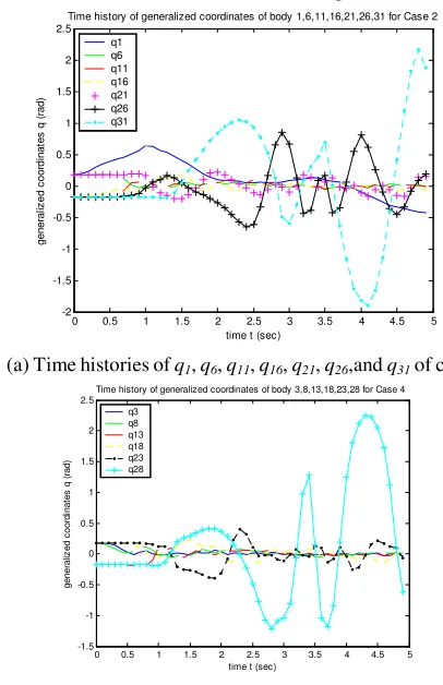
Figure 6 (a) and (b) show time histories of the generalized coordinates q1, q6, q11, q16, q21, q26,and q31 of case 2, and q3,

q8, q13, q18, q23, and q28 of case 4. These time history curves

agree with those produced by commercial dynamical analysis software Autolev. In figure 7, motion trace simulations associated with each body of each subchain for case 3 are given. From figure 7, it can be seen clearly that configurations of four subchains are updated in parallel. Due to constraints imposed between subchains being communicated correctly

during concurrent simulation, the motion of outboard tip of each proximal sub-

chain is exactly same as the motion of inboard tip of each distal subchain. If the motion trace of each subchain in figure 7 (a), (b), (c), (d) is superposed on another, the motion trace of the entire subchain can be obtained as in figure 7 (e).

0 0.5 1 1.5 2 2.5 3 3.5 4 4.5 5

-2 -1.5 -1 -0.5 0 0.5 1 1.5 2 2.5

time t (sec)

ge

ne

ra

liz

ed

c

oo

rd

in

at

es

q

(r

ad

)

Time history of generalized coordinates of body 1,6,11,16,21,26,31 for Case 2 q1

q6 q11 q16 q21 q26 q31

(a) Time histories of q1, q6, q11, q16, q21, q26,and q31 of case 2

0 0.5 1 1.5 2 2.5 3 3.5 4 4.5 5 -1.5

-1 -0.5 0 0.5 1 1.5 2 2.5

time t (sec)

ge

ne

ra

liz

ed

c

oo

rd

in

at

es

q

(r

ad

)

Time history of generalized coordinates of body 3,8,13,18,23,28 for Case 4

q3 q8 q13 q18 q23 q28

(b) Time histories of q3, q8, q13, q18, q23, and q28 of case 4

[image:5.612.332.520.120.275.2]

Figure 6: Time Histories of Generalized Coordinates Table 2 shows average time cost of a function evaluation of six cases with application of five Krylov subspace methods in Aztec to each case. Take case 4 as an example. From table 1 it is clear that there are 7 cuts and 8 processors for case 4. Each processor contains 4 bodies. In table 2, average time cost of a single function evaluation is 1.06e-3 seconds for CG, 1.17e-3 seconds for CGS, 1.17e-3 seconds for TGQMR, 1.15e-3 seconds for BiCGSTAB, and 1.1e-3 seconds for GMRES respectively.

Table 2: Average Time Cost of a Function Evaluation Time in Seconds

Krylov Method CG

CGS TFQMR BiCGSTAB GMRES

Case 1 4.7e-4 4.75e-4 4.7e-4 4.65e-4 4.7e-4 Case 2 5.4e-4 5.6e-4 5.7e-4 5.75e-4 5.55e-4 Case 3 9.2e-4 9.1e-4 9.35e-4 9.25e-4 9.3e-4 Case 4 1.06e-3 1.17e-3 1.17e-3 1.15e-3 1.1e-3 Case 5 1.23e-3 1.83e-3 1.73e-3 1.765e-3 1.54e-3 Case 6 2.34e-3 2.49e-3 2.51e-3 2.465e-3 2.39e-3 The time data from table 2 agree well with the theoretical estimation of computational cost as follows [10]:

(

1

)

log

₂

−

+

+

+

≈

p

p p p

N

m

N

m

N

nm

N

n

[image:5.612.73.298.546.632.2]

-8 -6 -4 -2 0 2 4 6 8 10 12 0

2 4 6 8 10 12 14 16

Motion trace of subchain 1 of case 3

x (m)

y

(m

)

subchain 1 contains body 1-8

initial position

-15 -10 -5 0 5 10 15 20 25 5

10 15 20 25 30

35

Motion trace of subchain 2 of case 3

x (m)

y

(

m

)

subchain 2 contains body 9-18

floating joint on base body due to cutting initial position

(a) subchain 1 (b) subchain 2

-15 -10 -5 0 5 10 15 20 25 30 0

5 10 15 20 25 30 35

Motion trace of subchain 3 of case 3

x (m)

y

(m

)

subchain 3 contains body 19-24 initial position floating joint on base body due to cutting

-15 -10 -5 0 5 10 15 20 25 5

10

15

20

25

30

Motion trace of subchain 4 of case 3

x (m)

y

(m

)

subchain 4 contains body 25-32

initial position floating joint on base body due to cutting

(c) subchain 3 (d) subchain 4

-30 -20 -10 0 10 20 30 40 50

0

10

20

30

40

50

60

Motion trace of entire chain of case 3

x (m)

y

(m

)

entire chain contains 32 bodies

(e) the entire chain Figure 7: Motion Trace of Case 3

V. CONCLUSIONS

A new HDIA procedure and its parallel implementation on IBM 1350 cluster via integration with various nonstationary iterative solvers in Aztec have been introduced in this paper. Joint separation is utilized to distributed computing loads in parallel so that five computational tasks associated with formation/solution of equation (1) and consequent integration for updating state variables can be carried out efficiently for parallel simulation. An efficient sequential O(n) method is utilized within each processor in parallel for formulation and solution of equations of motion (1a), and parallel techniques are applied between processors for formation and solution of constraint equation (1b). A combination of direct and iterative linear equation solution methods is created to achieve high overall computational efficiency. Thus the algorithm can fully offer advantages of both the sequential O(n) procedure and parallel computation. A computational complexity of

O

+

+

+

log

₂

(

_p

−

1

)

p p p

N

m

N

m

N

nm

N

n

γ γ

performance can be achieved with Np processors for a chain

system with n degrees of freedom and m constraints due to separation of interbody joints. The index

γ

is the parameter for iterative solver performance. It depends on effectiveness of the preconditioner, the quality of the solution initial guess, the eigenvalue spectra of the constraint force coefficient

matrix, and the convergence criteria used.

The integration of the HDIA with Krylov subspace iterative solvers in Aztec enhances the application power of HDIA so that it can handle various properties that constraint coefficient matrix in equation (1b) may have. Both the algorithm and its integration with Aztec have been validated and implemented on IBM 1350 with MPI. Various joint separation cases and iterative solvers have been used to show flexibility of HDIA.

ACKNOWLEDGMENT

Authors wish to acknowledge and thank financial support from SD NASA EPSCoR Research Initiative fund and SDSU Research Start-up grant.

REFERENCES

[1] H. Kassahara, H. Fujii, and M. Iwata, “Parallel Processing of Robot Motion Simulation”, Proc. IFAC 10th _{World Conference, Munich,} FRG, July, 1987.

[2] D. S. Bae, J. G. Kuhl, and E.J. Haug, “A recursive Formation for Constrained Mechanical System Dynamics: Part III, Parallel Processing Implementation,” Mechanisms, Structures, and Machines, Vol. 16, 1988, pp. 249-269.

[3] S. S. Lee, “Symbolic Generation of Equation of Motion for Dynamics/Control Simulation of Large Flexible Multibody Spaces Systems”, Ph. D. Dissertation, University of California at Los Angeles, 1988, UMI No. 8814809

[4] K. S. Anderson, 1990. “Recursive Derivation of Explicit Equations of Motion for Efficient Dynamic/Control Simulation of Large Multibody Systems.” Ph.D. Dissertation, Stanford University. UMI No. 9108778. [5] K. S. Anderson, “An Efficient Modeling of Constrained Multibody

Systems for Application with Parallel Computing,” Zeitschrift fur Angewante Mathematic un Mechanik, Vol. 73, No. 6, 1993, pp. 520-528.

[6] A. Fijany, and A. K. Bejczy, “Parallel Computation of Forward Dynamics of Manipulators”, JPL New Technology Report NPO-18706, NASA Technical Brief, Vol. 17, No. 12, Item 82, December 1993.

[7] I. Sharf, and G.M.T. D'Eleuterio, “An Iterative Approach to Multibody Simulation Dynamics Suitable for Parallel Implementation,” Journal of Dynamic Systems, Measurement and Control, Vol. 115, Dec. 1993, pp. 730-735.

[8] A. Fijany, I. Sharf, and G.M.T. D'Eleuterio, “Parallel O(log N)

Algorithms for Computation of Manipulator Forward Dynamics,”

IEEE Transactions on Robotics and Automation, Vol. 11, No. 3, June 1995, pp. 389-400.

[9] K. S. Anderson and S. Z. Duan, “A Highly Parallelizable Low Order Algorithm for Dynamics of Multi-Rigid-Body Systems: Part I, Chain Systems”, Journal Mathematical and Computer Modeling, Vol. 30, 1999, pp. 193-215

[10] Duan, S. Z. and K. S. Anderson, “Parallel Implementation of a Low Order Algorithm for Dynamics of Multibody Systems on a Distributed Memory Computing System”, Journal Engineering with Computers, Vol. 16, No. 2, 2000, pp. 96-108.

[11] R.S. Tuminaro, M. Heroux, S.A. Hutchinson, and J.N. Shadid,

Official aztec user's guide version 2.1. Massively Parallel Computing Research Laboratory, Sandia National Laboratories, Albuquerque, NM, 1999.

[12] T. R. Kane, and D. A. Levinson, 1985. Dynamics: Theory and Application. McGraw Hill, NY.

[13] S. Z. Duan, and Y. Patel, “A Hybrid Parallelizable Algorithm for Computer Simulation of the Motion Behaviors of a Branched Multibody System.” Proceedings of 2006 ASME International Conference and Exposition. Chicago. November 5-10, 2006. [14] S. Z. Duan, and J. A. Ries, “Efficient Parallel Computer Simulation of

the Motion Behaviors of Closed-loop Multibody Systems”

Proceedings of 2007 ASME International Mechanical Engineering Congress and Exposition, November 11-15, 2007, Seattle, Washington.

[15] Y. Saad, Iterative Methods for Sparse Linear Systems, PWS, Boston, 2000.