Abstract—Container throughput plays a major role in the development of operational strategies and long-term investment plans for container terminals. Support Vector Machine (SVM), as a powerful technique for regression and classification, shows impressive performance in the area of time series analysis. This paper presents a modified version of SVM, called the least squares support vector machine (LS-SVM), as an effective technique to forecast the monthly container throughput in Hong Kong. It also proposes a method for fast training LS-SVM by employing an approximate approach to accelerate the training process and lower the memory requirement. The proposed Approximate LS-SVM (ALSSVM) has a shorter training time than LS-SVM and a forecasting accuracy comparable to that of the standard SVM and the LS-SVM. To evaluate the effectiveness of ALSSVM, numerical experiments are conducted to compare its performance with that of standard SVM, LS-SVM and RBF Neural Network for forecasting Hong Kong’s container throughput. The results show that the proposed method is an excellent forecasting tool for logistics management.
Index Terms—Approximate LS-SVM, Container through- -put forecasting, Time series analysis.
I. INTRODUCTION
Hong Kong is the world’s 7th largest maritime centre with ship owners managing about 8% of the global merchant fleet and millions of tonnage of cargoes passing through its container terminals every year. In 2005, Hong Kong handled 22.6 million Twenty-foot Equivalent Units (TEUs) of containers resulting in a 2.8% increase year to year as compared to the 2004 throughput. Currently, the container terminals in Hong Kong, in aggregate, handles over 80 percent, by weight, of Hong Kong's trade, making them the busiest in the world. Containerization is a preferred form of transport for almost all imported/exported materials, components, and manufactured products. Its growth has a significant impact on container terminal operations, and has important implications on a container terminal’s future infrastructure requirements. Indeed,
Manuscript received March 6, 2007.
K.L. Mak is Professor at the Department of Industrial and Manufacturing Systems Engineering, The University of Hong Kong. (phone: (852) 28592582; e-mail: [email protected]).
D.H. Yang is a PhD student at the Department of Industrial and Manufacturing Systems Engineering, The University of Hong Kong. (e-mail: [email protected]).
container throughput forecast is playing an increasingly important role in container terminal management. However, it is commonly known that container throughput is affected by many varying factors, such as seasons, the amount of imports and exports, as well as general economic conditions. The complex nature of these factors and their dynamic interactions make precise forecasting of container throughput a long-term challenge. Hence, to better assist local terminal operators in developing operational strategies and investment plans, it is important to develop an efficient methodology for forecasting Hong Kong’s container throughput.
Support Vector Machine (SVM) proposed by Vapnik and his co-workers [1] is a classic algorithm for regression estimation and classification. In view of its successful applications in time series analysis [2,3], the technique has been used in numerous areas of forecasting, e.g. predicting the complex financial indexes [4] and random wind speed [5]. When combined with some heuristic algorithms, such as simulated annealing, SVM can adjust its hyper-parameters to achieve better forecasting results [6]. Moreover, SVM for classification can also be used to accomplish some predictions if the output outcome can be classified into binary category [7].
Usually, the training of a standard SVM involves the solution of a quadratic optimization problem with inequality constraints [1]. A traditional method is to solve the problem directly by using numerical optimization software [8]. However, this method is normally not satisfactory because of the low training speed and the large memory requirement when the amount of training data is huge. In order to facilitate application of the technique, LIBSVM [9] provides a library that implements several popular algorithms to solve SVM-related problems efficiently. Mostof these algorithms are computationally better than those adopted in other commercial optimization software. A modified version of SVM is the Least Squares SVM (LS-SVM) [10] which involves the solution of a quadratic optimization problem with a least squares loss function and equality constraints instead of inequality constraints. As a result, the constrained quadratic optimization problem can be converted into solving a set of linear equations that satisfy the Karush-Kuhn-Tucher (KKT) condition. Although LS-SVM is easily understood and programmed, the required storage and training time are 2
( )
O n and 3 ( ) O n , respectively, where n is the amount of training data involved. Hence, when n is large, the kernel matrix cannot be
Forecasting Hong Kong’s Container Throughput
with Approximate Least Squares Support Vector
Machines
accommodated in the memory and a large amount of computational effort would be required in the training process. To accelerate the training speed and lower the memory requirement, several approximate methods have been derived recently, which include the Incomplete Cholesky Factorization [11,12], the NYSTRÖM method [13], the Sparse Greedy Matrix Approximation [14], and the Reduced set vectors method [15]. The key essence of these approaches is to replace the kernel matrix with a lower rank version through some approximate techniques. It is commonly known that such kinds of approximate methods can largely improve the computational performance of kernel machines but do not lose their good generalization capability. Among these approximate methods, Incomplete Cholesky Factorization (ICF) is originally used for training SVM, a particular type of kernel machines, with an interior point algorithm [11]. The technique has been shown to possess good computational characteristics [16]. It builds a lower-rank rectangular matrix k(n m m× ( <n)) column by column in order to greedily decrease the trace of the residual matrix between the exact kernel matrix Hand the approximate
one T
K%=kk . This lowers the required storage from 2 ( ) O n to ( )
O mn and reduces the amount of computational load from 3
( )
O n to about 2
( 2)
O nm [11].
Sherman-Morrison-Woodbury (SMW) equation [12] which is a useful means for performing matrix inversion, can be employed to train an LS-SVM efficiently when the kernel map is explicitly known (e.g., the kernel function is linear or quadratic) [18]. However, this method cannot be directly applied to some nonlinear kernels (e.g., the RBF kernel). This paper therefore proposes an approximate method called ALSSVM for training an LS-SVM. It firstly uses ICF [11,12] to derive one rectangular matrix and to replace the kernel matrix in the LS-SVM by a lower-rank version. The SMW equation is then employed to solve the set of linear equations efficiently when numerical instability does not occur.
It is shown that the proposed Approximate Least Squares Support Vector Machines (ALSSVM) exhibits a good performance, when applied to forecast the Hong Kong’s container throughput. Compared to other machine learning algorithms, e.g. standard SVM, LS-SVM and RBF Neural Network, the proposed method performs very well in terms of fast computational speed and good prediction accuracy.
The remainder of the paper is organized as follows. Section
Ⅱ introduces the basic theory of LS-SVM for regression. Section Ⅲ shows the proposed approximate method, and to highlight the concepts of the Incomplete Cholesky Factorization approach and the Sherman-Morrison-Woodbury (SMW) equation. The application of the proposed method to forecast Hong Kong’s container throughput and the analysis of the results obtained are shown in Section Ⅳ. The conclusion is presented in Section Ⅴ.
II. LS-SVM FOR REGRESSION
In this section, we briefly introduce the basic theory of LS-SVM for regression [10]. Given a training set {(x , )} 1
n i yi i=
with inputs xi∈ d and outputsyi∈ , training the SVM for
regression is firstly to map the input data into a high-dimensional feature space by a kernel function that satisfies Mercer’s condition: K x x( ,i j)=φ( )xi φ(xj). Typical kernel functions include Linear K x x( , k)=x xTk ,
Polynomial K x x( , k)=(x xTk +1)d , RBF K x x( , k)=exp( 0.5− ∗ −x xk σ2) and MLP K x x( , k)=tanh[κx xkT +θ]. Then a linear regression is implemented in this high-dimensional feature space. The approximate function has the form:
( ) T ( )
f x =w φ x +b (1) where wand bare the coefficients and the bias, respectively, which can be estimated from the training data; φ( ) is the kernel mapping data from the input space into the feature space. In LS-SVM, the following constrained optimization problem is considered: 2 2 , , 1 min 2 2
. . ( ) , {1,... }
w b
T
i i i
C
s t φ x b y ξ i n
⎧ +
⎪ ⎨
⎪ + = − ∀ ∈
⎩
ξ w ξ
w
(2)
where ξi is the error variable, and C is the tradeoff parameter
adjusting the function complexity and the approximating errors. The most obvious feature of LS-SVM is that it uses the least square of error as the loss function, instead of the ε-insensitive loss function or Huber function as in the case of standard SVM for regression [1,8]. This feature allows the whole problem to be transformed from solving a quadratic programming problem to solving a set of linear equations. The Lagrangian function is given as: 2 2 1 1 ( , , , ) 2 2 ( ( ) ) n T
i i i i
i
C
L b
x b y
α φ ξ
=
= +
−
∑
+ + −w ξ α w ξ
w
(3)
The optimal solution of this problem is given by the Karush-Kuhn-Tucher (KKT) conditions, thus resulting in the following set of linear equations:
1
1
0 ( )
0 0
0 , {1,... }
0 ( ) 0, {1,... }
n i i i n i i i i i T
i i i
i L x w L b L
C i n
L
x b y i n
α φ α α ξ ξ φ ξ α = = ⎧ ∂ = ⇒ = ⎪ ∂ ⎪ ⎪ ∂ ⎪ = ⇒ = ⎪⎪∂ ⎨ ⎪ ∂ = ⇒ = ∀ ∈ ⎪∂ ⎪ ⎪ ∂ = ⇒ + + − = ∀ ∈ ⎪ ∂ ⎪⎩
∑
∑
w w (4)0
0 T b
⎡ ⎤ ⎡ ⎤ ⎡ ⎤= ⎢ ⎥ ⎢ ⎥ ⎢ ⎥ ⎣ ⎦ ⎣ ⎦
⎣ ⎦
1
α y
1 H (5) where y=[ ;y y1 2; ...;yn] denotes the column vector formed
by the outputs of the training points. The matrixHis defined by ( , )
ij i j ij
h =K x x +δ C where δij denotes the Kronecker delta. Since the matrix at the left side of equation (5) is not positive definite, equation (5) can not be solved by iterative methods efficiently. Similar to the LS-SVM for classification [17], the problem can be reformulated as solving the equation
1
1
0 ( )
0
T
b s
b
α
− −
⎡ ⎤ ⎡ ⎤
⎡ ⎤ =
⎢ ⎥ ⎢ ⎥
⎢ ⎥ +
⎣ ⎦ ⎣ ⎦ ⎣ ⎦
1 H y
H H 1 y (6) where
1
( ) 0
T
s=1 H 1− > (7) In this case, the coefficient matrix of the linear system is a positive definite matrix that allows the use of existing numerical optimization methods to solve equation (6). Also, the solution of equation (6) can be found by using the following three steps:
Step 1: Step 2: Step 3:
s
b s
b ⎧
⎨ ⎩ = ⎧ = ⎪ ⎨
= − ⎪⎩
N
T
T Hη= 1
Hν= y 1 .η
η.y
α ν η
(8)
Step 1 is the most important step, which consumes a large percentage of the computational effort. The solution complexity is equal toO n( 3), indicating that large amount of computational effort will be required when the training number becomes huge. Although an existing optimization method, e.g. the conjugate gradient algorithm, can be used to solve equation (6), a huge data set still cause problems in memory storage and long training time. Hence, it is necessary to develop an efficient method to overcome these difficulties.
III. DEVELOPMENT OF METHODOLOGY A. Incomplete Cholesky Factorization
The above discussion clearly shows that the conventional LS-SVM runs into two difficulties caused by the large but not sparse coefficient matrix. To alleviate these difficulties, some approximate methods have been proposed recently, which include the Incomplete Cholesky Factorization (ICF) [11,12], the NYSTRÖM method [13], the Sparse Greedy Matrix Approximation [14] and the Reduced vectors method [15], to replace the exact kernel matrix with an approximate version. In view of the excellent results displayed by ICF in a previous
experimental study [16], the method is adopted in this paper to provide an approximate version of the coefficient matrix. The procedure is outlined in the next few paragraphs.
Any positive definite matrix Qcan be represented by its Cholesky factorization T
Q=qq , where q is a lower triangular matrix [11,12]. If Q is positive semi-definite and singular, it is still possible to compute an “incomplete” Cholesky factorization T
qq , where some columns of q are zero. Choosing an appropriate threshold value, the procedure can also produce a rectangular matrix q ( n m m× ( <n) ) by pruning the column corresponding to the pivots that are below the threshold. This method can achieve a small numerical error and a good approximation to original matrix.
In view of the above argument, Fine and Scheinberg [11] have derived a method to construct the approximate kernel matrix Q% by directly approximating the Cholesky factorization of Qwith symmetric permutations. This method is a column by column process to obtain the rectangular matrix. In each iteration, greedy strategy and pivoting technique are used to obtain the best reduction of the trace of the residual matrix. Then one of subsequent columns is updated as the normal Cholesky factorization. The algorithm developed has complexity of 2
( )
O m n . The general description of the algorithm is shown in Fig. 1 and its details can be found in [11].
2 Input : , ,
(*,*) and
;
update the elements in ; ( )
select the maximum one from ;
pivot both the rows and columns of thefactorized columns;
( ) ;
( , )
n m tol
Kernel
while column m
column ++
TRACE
if tr Q tol
TRACE
p column
q column column sqrt
σ
θ
θ
<
Δ >
=
= (max( ));
( : , ) ( : , );
update ( : , ) as normal Cholesky factorization;
Output : and
note : 1) is a matrix;
2) is an array to record the trace of residual matrix; 3
TRACE
q column n column Kernel column n column q column n column
end end
q p
q n m
TRACE
=
×
[image:3.612.46.296.193.270.2]) pis an array to record pivoting sequence.
Fig. 1 Incomplete Cholesky Factorization algorithm
B. Sherman-Morrison-Woodbury (SMW) update
After the establishment of the low-rank approximate matrix
T
factorization update. However, it may experience numerical instability when the condition number of the matrix is sufficiently large. In LS-SVM, the coefficient matrix in (8) is positive definite, although it may become positive semi-definite when C goes to infinity. Generally, when C is not very large, the condition number of the matrix should not be large enough to make SMW update engenders obvious numerical instability. Therefore, the SMW equation is applied to conduct the matrix inversion here because of its fast speed and it is introduced in the following section.
In some cases, when a matrix G% is found to approximate the original matrix G , it may be factorized as T
G%=XBX , whereG% is an approximate matrix whose rank ism m( <n), X is a n m× matrix, B is an identity matrix [11] or a diagonal matrix with the diagonal entries equal to eigenvalues of a sub-matrix [13]. The Sherman-Morrison-Woodbury (SMW) equation
1 1 1 1 1 1 1
( T) ( T ) T
A+XBX − =A− −A X B− − +X A X− − X A− (9) can then be used to update the inverse of the low-rank matrix [12].
When the SMW equation is used to solve the set of linear equationsH%α β= , the n n× approximate kernel matrix H% can be expressed as ( + T)
A XBX . Hence, the solution α is given by
1 1
( )
α β
γ μ
−
− = + = −
T
A XBX
A X (10) where
1
A γ = −β
(11)
1 1
: (B X A XT ) XT μ = − + − μ= γ
(12) This also indicates that only the diagonal matrices A and B, and matrix X need to be stored in the memory, not the matrix
H%[11].
The m m× matrix (B−1+X A XT −1 ) in equation (12) is symmetric positive definite and can be solved by using Cholesky factorization which has a complexity of 3
( ) O m . The time complexity of the overall work required to solve H%α β= is about 2
( 2)
O nm [11]. C. Approximate LS-SVM
The procedure of the proposed Approximate Least Square Support Vector Machine is outlined below:
Step 1: Select the rank (m) of the approximate matrixK% ; Step 2: Generate a rectangular matrix k n m( × )with ICF to
approximate the kernel matrix K such that
T K≈K%=k k;
Step 3: Use the SMW equation to solve the first two sets of equations given by the step 1 of equation (8);
Step 4: Obtain the solution by using the last two steps of equation (8).
IV. CONTAINER THROUGHPUT FORECASTING A. Container Data Collection
As container throughput greatly influences the operational strategies and investment plans of a container terminal, it is important to provide container terminal operators in Hong Kong with an efficient method to forecast Hong Kong’s container throughout. In order to validate the effectiveness of the various forecasting models, this study has collected the historical data of container throughout in Hong Kong from the Marine Department of Hong Kong SAR of PR China. The whole data set covers the period from January 1995 to October 2006, totally 142 observations.
B. System Analysis
This study views the Hong Kong’s container throughout value as a time series data stream. Hence, if the embedded dimension is h and the time-delay isτ , the next output value is predicted on the base of the previous h consecutive data as follows:
( 1) ( ( )), 1, 2,...,
X k+ = f X k k= n
where
( ) [ ( ), ( ),..., ( ( 1) )]T X k = x k x k−τ x k− −h τ .
All data are normalized into the range of [0, 1] in order to utilize the dataset effectively. The embedding dimension is set to 12, which corresponds to the seasonal trend. As a result, the data set is processed to obtain 142-12 = 130 groups of data with each group of data expressed as a 12-d vector. The processed set is then divided into three parts. The first part contains the first 90 data for training the SVM model. Since the RBF kernel is employed in the analysis, training the SVM model needs to determine two more parameters: the tradeoff parameter C for complexity adjustment and the bandwidth parameter σ2
for the RBF kernel. The second part includes the next 20 data to be used to determine these two model parameters. The optimal pair of C and σ2
are obtained by grid searching [15,17]:
3 2 0 9 10
{2 , 2 ,..., 2 ,..., 2 , 2 }
C∈ − − and 2 5 0 9
{2 ,..., 2 ,..., 2 }
σ ∈ −
. The total number of parameter pair is 14 15× =210 . A pair of optimal parameters is obtained when the model has achieved the highest validation accuracy. The last 20 data is reserved for testing the prediction accuracy and comparing the performance of the various models.
parameters are determined when the validation data set achieves the best predictive result. The rank of the approximate matrix of the proposed ALSSVM is set to 15.
Fig. 2 Forecasting result of ALSSVM
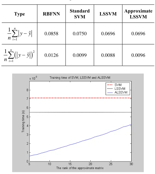
[image:5.612.48.296.432.710.2]The various models are trained by using all 90 data in the first part and evaluated by using the 20 data in third part of the dataset. Fig 2 shows the actual throughput value in the whole dataset and the forecast produced by using the proposed method. Table 1 compares the performances of the various methods in terms of two criteria, namely, the Mean Absolute Error (MAE) and the Mean Square Error (MSE). To compare the training speed, the SVM and the LS-SVM are executed 500 times to determine the average training time. The proposed ALSSVM is also executed 500 times to determine the average training time for each rank of the approximate matrix. The final results are shown in Fig 3.
Table 1. Forecasting Error of Different Models
Type RBFNN Standard SVM LSSVM Approximate LSSVM
1 1 n
i
y y n =
−
∑
% 0.0858 0.0750 0.0696 0.0696(
)
21 1 n
i
y y n =
−
∑
% 0.0126 0.0099 0.0088 0.0096Fig. 3 Training time of SVM, LS-SVM and ALS-SVM
The results listed in Table 1 indicate that all four methods can achieve good and similar results for forecasting the Hong Kong’s container throughput. The forecasting accuracy of LSSVM and ALSSVM are close to that of the standard SVM, but better than that of RBFNN. Moreover, the curves in Fig.3 show that the average training time of ALSSVM is almost proportional to the rank of the approximate matrix, and is significantly shorter than that of SVM and LSSVM.
V. CONCLUSION
Information concerning container throughput is important for container terminal operators in Hong Kong in making operational strategies and investment plans. This paper has proposed a method, called Approximate Least Squares Support Vector Machines (ALSSVM), to forecast Hong Kong’s container throughput. The method uses the Incomplete Cholesky Factorization technique and the Sherman-Morrison- Woodbury (SMW) equation to alleviate the difficulty related to memory storage and to improve the training speed. The results of applying ALSSVM to past container throughput data obtained from the Marine Department of HKSAR clearly demonstrate that the proposed method is an effective and efficient forecasting tool. In addition, comparison of the performances of ALSSVM, LSSVM, standard SVM and RBF neural network shows that ALSSVM, LSSVM, standard SVM exhibit similar performances which are better than RBF neural network, and ALSSVM is better than SVM and LSSVM in terms of computational speed.
REFERENCES
[1] Vapnik, V.1995. The Nature of Statistical Learning Theory. Springer-Verlag.
[2] K.R. Müller, A.J. Smola, G.Rätsch, B. Schölkopf, J. Kohlmorgen, and V.Vapnik. “Using support vector machines for time series prediction”. Advances in kernel methods: support vector learning. 1999, pp. 243-253. [3] S. Mukherjee, E. Osuna, and F. Girosi. “Nonlinear prediction of chaotic time series using support vector machines”. Proceeding of IEEE NNSP 97, Smelia Island, FL, 24-26, Sep., 1997.
[4] F.E.H. Tay, L Cao. “Application of support vector machines in financial time series forecasting”. Omega, Vol. 29, 2001, pp. 309-317.
[5] M.A. Mohandes, T.O. Halawani, S. Rehman, and A. A. Hussain. “Support vector machines for wind speed prediction”. Renewable Energy. 29: 939–947, 2004.
[6] P.F. Pai and W.C. Hong. “Support vector machines with simulated annealing algorithms in electricity load forecasting”. Energy Conversion and Management. 46: 2669-2688. 2005.
[7] W. Huang, Y. Nakamori and S.Y. Wang, “Forecasting stock market movement direction with support vector machine”. Computers & Operations Research. 32: 2513-2522. 2005.
[8] S. R. Gunn. “Support vector machines for classification and regression”. Technical Report. University of Southampton. 10 May 1998.
[9] C.C. Chang and C.J. Lin. “LIBSVM: a library for support vector machines”. http://www.csie.ntu.edu.tw/~cjlin/libsvm/. 2004.
[10] J.A.K. Suykens, J.De Brabanter, L.Lukas and J. Vandewalle. “Weighted least squares support vector machines--robust and sparse approximation”. Neurocomputing. Vol. 48, pp. 85-105.
[11] S. Fine and K. Scheinberg. “Efficient SVM training using low-rank kernel representations”. Journal of Machine Learning Research, 2:243–264, Dec. 2001.
[13] C. K. I. Williams and M. Seeger. “Using the Nyström method to speed up kernel machines”. Advances in Neural Information Processing Systems, pp. 682–688. MIT Press, 2001.
[14] A. Smola and B. Schölkopf. Sparse greedy matrix approximation for machine learning. In Proc. Int’l Conf. Machine Learning, pages 911–918. Morgan Kaufmann, 2000.
[15] K.M. Lin and C.J. Lin. “A study of reduced support vector machines”. IEEE Transactions on Neural Networks. Vol. 14: 6. pp. 1449 – 1459. Nov. 2003.
[16] K.L. Mak and D.H. Yang. “Comparing Approximating Techniques in Least Square Support Vector Machines”. Technical Report. The University of Hong Kong. Aug. 2006.
[17] T. Van Gestel, J.A.K. Suykens, B. Baesens, S. Viaene, J. Vanthienen, G. Dedene, B. De Moor, J. Vandewalle. “Benchmarking least squares support vector machine classifiers”. Machine Learning, Vol. 54, Issue 1, pp. 5 – 32. Jan. 2004.