Simulation of Flow over a Car using Wind Tunnel
V. Guru shanker1, K. Vijay kumar2, Akella Shiva Subrahmanya Sai3
1, 2
Asst. Professor in Mechanical Engineering Department, Vignan Institute of technology & Science, India
3
U G Student, Mechanical Engineering Department, Vignan Institute of technology & Science, India
Abstract: Evaluation of the safety and performance of automobiles in windy conditions requires accurate descriptions of wind loads on vehicles. In this, “Aerodynamics” plays vital role in designing of any automotive. Due to the aerodynamics, the entire performance of the vehicle will be changed, like it improves the efficiency and reduces the fuel consumption, etc. In the present work we are considered a car model of Maruthi-Alto with slight modifications is designed and fabricated with wood and that model was tested in wind tunnel at different flow speeds and different ground clearances and calculated the aerodynamic characteristics. The experimental results divulge that the flow conditions did have effects on the variation of wind loads.
Keywords: Aerodynamics, Wind tunnel, Lift, Drag, Center of Pressure
I. INTRODUCTION
In order to evaluate the accident risks and stability for road vehicles under windy conditions, the aerodynamic loads gives the essential information to carry out the evaluation. Various approaches can be adopted to evaluate the wind loads on vehicles. Due to the difficulties in computational fluid dynamics and the expense involved in full-scale measurements, a wind tunnel study is probably the most convenient and reliable approach to examine this problem[1]. Data of aerodynamic loads on a double deck bus provided by Garry (1984) were quoted by Baker (1986), who performed wind tunnel tests with a 1/12-scaled model of a Leyland Altantaean bus.
It was noted that the effects of atmospheric turbulence and model/ground relative motion were not modeled for the tests, and the accuracy of these results were in doubt. In order to assess the effect of high winds on traffic in general, several standard types of vehicles were defined in alater study by Baker (1987), including cars, large rigid vans, and articulated tractor–trailers. In both of the above studies, the six aerodynamic coefficients were given in a simplified formula format. While comparisons of the Large Van category and Leyland Altantean Bus category in these two different studies show that they have very similar geometric parameters, the aerodynamic loads have significant difference.
In order to study the behavior of high-side vehicles in cross wind, Baker (1988) carried out a wind tunnel study on a 1/25 scale articulated lorry model, using a low turbulence flow and a static setup. The test results for the aerodynamic force coefficients were fitted with simple analytical curves[2], [3].
The comparison of this formulation to the earlier mentioned study (Baker 1987) show close values and similar trends in some cases, but also significant difference of magnitudes in other cases[5]. The present work is to check the performance of the car at different ground clearances and effect of mean wind loads on it at different speeds by altering some of its dimensions and scaling down the model and testing it in wind tunnel.
Wind tunnels enable the data like aerodynamic forces; drag, lift, side force and surface pressure distribution. Depending on the size of the vehicle and the limitations of the test facility models typically lie between 30% - 60%. Model scale testing is ideal for rapid evaluation of the influence of different body styles and features on the vehicle's aerodynamics.
II. DESIGN&FABRICATION
Fig. 1 Car model
III. EXPERIMENTALANALYSIS
[image:2.612.198.418.320.405.2]After obtaining the desired shape of a car model, is mounted vertically in the wind tunnel.A groove is made into the center of model and, Probes are fixed to the specimen by using POP as adhesive. The pressure tubes (13 with locations indicated) from the midpoint of car are connected to the inlet nipples of the tunnel pressure transducer array sampling system. The stationary pressure of the test section is connected to the reference connection of the pressure transducer. Testing of model is done at different speeds, ground clearance of 12 mm, as shown in fig. 2.
Fig. 2 Arrangement of Prototype in test section
IV. CALCULATIONS & RESULTS
For conversion to lift, drag, coefficients of model has a span width b= 13.525" and a chord length of c = 22.37". Normal Coefficient, N= N'*.9504-A'*.0082-P'*0.0161,Axial Coefficient, A = N'*.0608+A'*.5912
Pressure Coefficient, P= -N'*.1336+A'*.0119+P'*1.182, Coefficient of Drag = A cos α + N sin α, Coefficient of Lift = N cos α - A
sin αCp= (P-P_ref)/q_∞
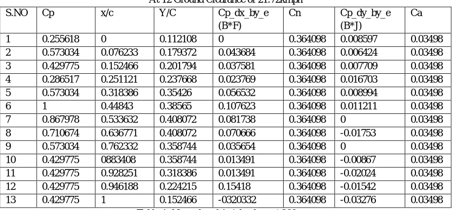
At 12 Ground Clearance of 21.72kmph
S.NO Cp x/c Y/C Cp_dx_by_e
(B*F)
Cn Cp_dy_by_e
(B*J)
Ca
1 0.255618 0 0.112108 0 0.364098 0.008597 0.03498
2 0.573034 0.076233 0.179372 0.043684 0.364098 0.006424 0.03498
3 0.429775 0.152466 0.201794 0.037581 0.364098 0.007709 0.03498
4 0.286517 0.251121 0.237668 0.023769 0.364098 0.016703 0.03498
5 0.573034 0.318386 0.35426 0.056532 0.364098 0.008994 0.03498
6 1 0.44843 0.38565 0.107623 0.364098 0.011211 0.03498
7 0.867978 0.533632 0.408072 0.081738 0.364098 0 0.03498
8 0.710674 0.636771 0.408072 0.070666 0.364098 -0.01753 0.03498
9 0.573034 0.762332 0.358744 0.035654 0.364098 0 0.03498
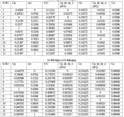
[image:2.612.75.539.512.727.2]At 500 Rpm (64.91 kmph)
S.NO Cp x/c Y/C Cp_dx_by_e
(B*F)
Cn Cp_dy_by_e
(B*J)
Ca
1 -0.4509 0 0.11211 0 0.10272 -0.0152 -0.0586
2 0.26012 0.0762 0.17937 0.02275 0.10272 0.00292 -0.0586
3 0 0.1525 0.20179 0 0.10272 0 -0.0586
4 -0.2139 0.2511 0.23767 -0.0211 0.10272 -0.0125 -0.0586
5 0.3237 0.3184 0.35426 0.03484 0.10272 0.00508 -0.0586
6 1 0.4484 0.38565 0.09417 0.10272 0.01121 -0.0586
7 0.6474 0.5336 0.40807 0.07403 0.10272 0 -0.0586
8 0.47977 0.6368 0.40807 0.05916 0.10272 -0.0118 -0.0586
9 0.39306 0.7623 0.35874 0.03261 0.10272 0 -0.0586
10 0.21387 0.8834 0.35874 0.00671 0.10272 -0.0043 -0.0586
11 0.21387 0.9283 0.31839 0.00767 0.10272 -0.0101 -0.0586
12 0.21387 0.9462 0.22422 -0.1012 0.10272 -0.0077 -0.0586
13 0.21387 1 0.15247 -0.1069 0.10272 -0.0163 -0.0586
At 900 Rpm (119.36kmph):
S.NO Cp x/c Y/C Cp_dx_by_e
(B*F)
Cn Cp_dy_by_e
(B*J)
Ca
1 -0.44379 0 0.112108 0 0.214225 -0.01493 0.06648
2 0.39645 0.0762 0.179372 0.030223 0.214225 0.004445 0.06648
3 0.029586 0.1525 0.201794 0.002587 0.214225 0.000531 0.06648
4 -0.17751 0.2511 0.237668 -0.01473 0.214225 -0.01035 0.06648
5 0.053254 0.3184 0.35426 0.005254 0.214225 0.000836 0.06648
6 1 0.4484 0.38565 0.107623 0.214225 0.011211 0.06648
7 0.674556 0.5336 0.408072 0.063523 0.214225 0 0.06648
8 0.467456 0.6368 0.408072 0.053453 0.214225 -0.01153 0.06648
9 0.408284 0.7623 0.358744 0.050349 0.214225 0 0.06648
10 0.260355 0.8834 0.358744 0.021599 0.214225 -0.00525 0.06648
11 0.260355 0.9283 0.318386 0.008173 0.214225 -0.01226 0.06648
12 0.260355 0.9462 0.224215 0.00934 0.214225 -0.00934 0.06648
[image:3.612.71.543.84.528.2]13 0.260355 1 0.152466 -0.12317 0.214225 -0.01985 0.06648
Table 3: Normal and Axial values at 900 rpm
A. Plotted Graphs
RPM Cd Cl
At 12mm Clearance
200 0.0001 -0.0005
500 -0.064 0.0783
Fig. 3 Clvs Cd for car model
The fig. 3 shows the minimum drag coefficient (Cd min) and can be calculated from data, fore body drag is 65% of coefficient of
drag, this is caused by over pressure on front face and this is reduced by accelerating the flow rounding up of upper horizontal and vertical leading edges, slanting the front face. Base drag is 34.9% of coefficient of drag Depression on the rear end and this is reduced by Increase of pressure: boat-tailing, tapering the rear part of the body, rounding up of trailing edges Side wall drag is 0.1% of coefficient of drag roof and underbody drag and this is caused by Shear stresses over the walls, roof and underbody and this can be reduced Decrease of shear stresses: reduction of roughness, decrease of the velocity in the underbody gap.
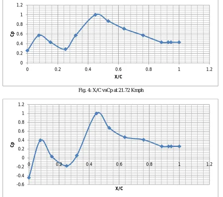
Fig. 4: X/C vsCp at 21.72 Kmph -0.05
0 0.05 0.1 0.15 0.2 0.25
-0.08 -0.06 -0.04 -0.02 0 0.02
C
l
Cd
0 0.2 0.4 0.6 0.8 1 1.2
0 0.2 0.4 0.6 0.8 1 1.2
C
p
X/C
-0.4 -0.2 0 0.2 0.4 0.6 0.8 1 1.2
0 0.2 0.4 0.6 0.8 1 1.2
C
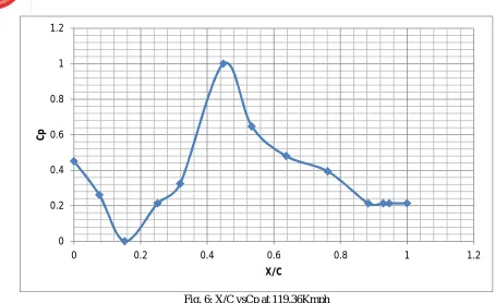
[image:4.612.83.532.322.719.2]Fig. 6: X/C vsCp at 119.36Kmph
V. CONCLUSION
Due to the aerodynamics the entire performance of the automotive will be changed in this work we designed a Car model and have been fabricated with wood considering its external geometry. Then the model has been tested in wind tunnel. The external flow for the car has been carried out at various speeds like 21.72 kmph, 64.9 kmph, and 119.6kmph. From the both analysis the aerodynamic characteristic has been studied. The experimental results reveal that the flow conditions have effects on the variation of wind loadsthere are better drag and lift positions which helps to increase the performance of the vehicle and also helps increase fuel efficiency.
REFERENCES
Journal Papers
[1] Baker, C.J., 1986.Asimplified analysis of various types of wind induced road vehicle accidents. J.WindEng.Ind.Aerodyn.22,69–85. [2] Baker,C.J., 1987.Measurestocontrolvehiclemovementatexposedsitesduring windy periods.J.WindEng.Ind.Aerodyn.22,151–161. [3] Baker, C.J.1988.Highsidedarticulatedroadvehiclesinstrongcrosswinds.J.Wind Eng. Ind.Aerodyn.31,67–85.
[4] Baker, C.J.1991.Groundvehiclesinhighcrosswinds.1.Steadyaerodynamicforces. J. FluidsStruct.5,69–90. [5] Coleman, S.A., Baker,C.J.,1990.Highsideroadvehiclesincrosswinds.J.WindEng. Ind. Aerodyn.36(2),1383–1392.
0 0.2 0.4 0.6 0.8 1 1.2
0 0.2 0.4 0.6 0.8 1 1.2
C
p
[image:5.612.71.525.61.339.2]