Abstract–CFD simulations of VAWT operation in unsteady wind conditions have been conducted. Validation of the numerical model was carried out by comparison to experimental data of a wind tunnel scale rotor. The performance of the VAWT under fluctuating winds was investigated and results show a dependency to Reynolds number. Increasing wind speeds cause blade lift to increase more rapidly than drag resulting to higher torque values. Deviation of instantaneous rotor CP from steady wind performance curve was seen. Rotor cycle CP matches steady wind values at the corresponding mean tip speed ratio.
Index Terms–unsteady wind, VAWT, CFD, wind tunnel
I. INTRODUCTION
he ill–effects of climate change have been becoming more severe and prevalent over the last decade or so [1]. The cause has been identified as greenhouse gas emissions from the burning of fossil fuels. For this reason, there has been a pressing need to reduce emissions through the use of technologies that are capable of extracting energy from the environment whilst being non–polluting and sustainable. Several alternative sources to fossil fuels have been identified with wind as one of the most promising. The contribution of wind to the total energy generation of the U.K. has been steadily rising over the last few years and has seen the greatest increase in 2011 of 68% for offshore installations and 45% for onshore [2]. Wind has also been the leading renewable technology for electricity generation with 45% of the total 2011 renewable production. Despite these numbers, the total consumption of electricity from renewable sources only account for 9.4%. As a result,
Manuscript received 1 March 2013, accepted 27 March 2013. This work was supported by the University of Sheffield Studentship Program, the Tertiary Education Trust Funds (TETFunds) of Nigeria through the Delta State Polytechnic, Ozoro and the Engineering Research and Development for Technology Program of the Department of Science and Technology through the University of the Philippines’ College of Engineering.
L. A. Danao, PhD is an Assistant Professor at the Department of Mechanical Engineering, University of the Philippines, Quezon City, Philippines (+63-2-9818500 loc 3130, [email protected]).
J. M. Edwards, PhD is a Research Associate at the Department of Civil and Structural Engineering, University of Sheffield, Sheffield, UK ([email protected]).
O. Eboibi is a PhD Student at the Department of Mechanical Engineering, University of Sheffield, Sheffield, UK ([email protected]).
R. Howell, PhD is a Lecturer in Experimental Aerodynamics at the Department of Mechanical Engineering, University of Sheffield, Sheffield, UK ([email protected]).
further research is needed to increase the understanding of this renewable power source to promote its wider adoption.
Much of the work on vertical axis wind turbine (VAWT) research is focused on steady wind conditions. If their use is to be successful, current efforts related to small scale VAWT should concentrate more on unsteady wind performance. VAWTs have been identified as the appropriate technology for urban wind generation where the nature of the wind flows is generally unsteady.
Earlier attempts to understand the performance of VAWTs in unsteady wind were carried out by McIntosh et al [3, 4] through numerical modelling. The VAWT was subjected to fluctuating free stream of sinusoidal nature while running at a constant rotational speed. An over–speed control technique resulted to a 245% increase in energy extracted while a tip speed ratio feedback controller incorporating time dependent effects of gust frequency and turbine inertia gives a further 42% increase in energy extraction. Danao and Howell [5] conducted CFD simulations on a wind tunnel scale VAWT in unsteady wind inflow and have shown that the VAWT performance generally decreased in any of the tested wind fluctuations. The amplitude of fluctuation studied was 50% of the mean wind speed and three sinusoidal frequencies were tested: 1.16Hz, 2.91Hz, and 11.6Hz where the fastest rate is equal to the VAWT rotational frequency. The two slower frequencies of fluctuation showed a 75% decrease in the wind cycle mean performance while the fastest rate caused a 50% reduction. In 2012, Scheurich and Brown [6] published their findings on a numerical model of VAWT aerodynamics in unsteady wind conditions. Different fluctuation amplitudes were investigated for three blade configurations: straight, curved, and helical. Constant rotational speed was used in the numerical simulations and the boundary extents were far enough for the model to be considered as open field. Helical blades perform much better with the unsteady CP tracing the steady performance curve quite well. Overall performance degradation is observed when fluctuation amplitudes are high while the effect of frequency is minor for practical urban wind conditions.
The research described in this study includes the development of a CFD–based numerical model, presented and validated against experiments to aid in the analysis of how and why a VAWT performs as it does in unsteady wind.
The Performance of a Vertical Axis Wind
Turbine in Fluctuating Wind –
A Numerical Study
Louis Angelo Danao, Jonathan Edwards, Okeoghene Eboibi, Robert Howell
1II. NUMERICAL MODEL OF THE WIND TUNNEL VAWT
The CFD package, Ansys Fluent 13.0, was used for all the simulations performed in this study. The coupled pressure–based solver was chosen with a second order implicit transient formulation for improved accuracy. All solution variables were solved via second order upwind discretisation scheme since most of the flow can be assumed to be not in line with the mesh [7]. The inlet turbulence intensity was set to Tu = 8% with a turbulence viscosity ratio of μt/μ = 14. These values were selected as they produced a turbulence intensity decay that is very close to the observed decay in experiments carried out by the authors. A two–dimensional CFD model was used to represent the VAWT and the wind tunnel domain. Based on the review of relevant literature [5, 8-19], it has been shown that a 2D model is sufficient in revealing the factors that influence the performance and majority of flow physics that surround the VAWT.
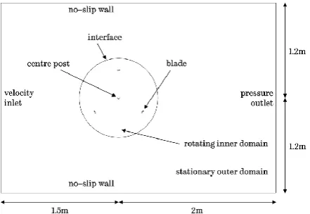
[image:2.595.316.542.537.716.2]The VAWT studied was a 3–bladed Darrieus rotor with a NACA0022 blade profile. The blade chord c was set to 0.04m with a rotor radius equal to 0.35m. A centre post with a diameter of 0.025m was placed in the rotation axis. The domain mesh was created around each aerofoil and the surrounding wind tunnel geometry was defined based on studies of the extents of the boundaries. There is an inner circular rotating domain connected to a stationary rectangular domain via a sliding interface boundary condition that conserves both mass and momentum. No–slip boundaries are set to represent the wind tunnel walls while a velocity inlet and a pressure outlet are used for the test section inlet and outlet, respectively. Each blade surface was meshed with 300 nodes and clustering in the leading and trailing edges was implemented. A node density study of five settings was the basis for the final surface mesh. The O–type mesh was adapted for the model, where a boundary layer was inflated from the blade surface. The first cell height used was such that the y+ values from the flow solutions did not exceed 1. Beyond the blade surface of about a chord width, the rotating inner domain mesh was generated such that the maximum edge length of the cells did not exceed 0.5c within the VAWT domain. The mesh was smoothed to reduce the angle skewness of the cells such that the maximum was observed to be less than 0.6.
Figure 1. An illustration of the 2D numerical domain.
The domain extents were also selected from a series of sensitivity tests to determine the appropriate distance of the walls, inlet and outlet boundaries from the rotor. The final wall distance from the rotor axis was set to 1.2m while the inlet was placed at 1.5m from the rotor axis with the outlet placed at 2m from the rotor axis (Figure 1).
Sufficient temporal resolution is necessary to ensure proper unsteady simulation of the VAWT. Different time step sizes Δt that are equivalent to specific rotational displacements along the azimuth were tested. The chosen time step size was Δt = 0.5°ω–1 which properly captures the vortex shedding and stalling at critical λ’s.
Time step convergence was monitored for all conserved variables and it was observed that acceptable levels of residuals (less than 1 × 10⁻⁶) were attained after 6 rotations of the VAWT. This meant that periodic convergence was also achieved. The blade torque Tb monitored all though 10 rotations. After the sixth rotation, the peaks of the upwind torque for cycles 7 through 10 are level and the downwind ripple match closely. The difference in average torque between cycle 7 and cycle 10 is around 0.5%.
IV. VALIDATION OF CFDMODEL
The numerical model developed was checked against experimental data to assess its capability of correctly simulating VAWT flow physics. The first aspect of the model validation is the comparison of the predicted VAWT performance over a wide range of operating speeds. The Transition SST model was tested against the experimentally derived CP. The steady wind speed was 7m/s and the simulations were run at different tip speed ratios from λ = 1.5 up to λ = 5 in increments of 0.5. The numerical model over–predicts CP starting from λ = 2 all the way up to λ = 5 (Figure 2). Maximum CP is 0.33 at λ = 4.5. Higher λ’s show the greatest over–prediction of the CFD model from experiments. This may be due to the effects of finite blade span where the reduction in aspect ratio as seen by McIntosh [20] cause a substantial drop in CP at high λ versus the small drop in CP at low λ.
Figure 2. Steady CP curves at 7m/s.
[image:2.595.61.282.590.742.2]to published data by Raciti Castelli et al [15], Howell et al [13] and Edwards et al [11] where 2D CP is over–predicted over the entire range of λ. Overall, the general trend of the predicted CP matches well with the experimental data. There is an observed negative trough at the low λ which rapidly rises and reaches maximum values near the experiment maximum at λ = 4 after which a rapid drop in CP is seen.
The second aspect of validation is the comparison of flow visualisations between CFD and PIV. The flow physics at two λ are inspected and assessed to determine the most appropriate turbulence model is used based on the accuracy of the predicted stalling and reattachment of the flow on the blades as they go around the VAWT.
θ CFD : Trans SST PIV
60°
[image:3.595.48.288.231.468.2]90°
Figure 3. Flow visualisations of vorticity in the upwind for λ = 2.
θ CFD : Trans SST PIV
130°
18
0°
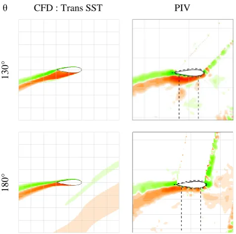
[image:3.595.48.287.491.728.2]Figure 4. Flow visualisations of vorticity in the downwind for λ = 4.
Figure 3 shows the vorticity plots for the upwind at λ = 2. Flow is observed to be attached until θ = 60° where both the Transition SST model and PIV reveal a bubble that is forming on the suction surface of the blade. The subsequent vortex shedding of the numerical model is seen to be in sync with the PIV. Flow visualisations for λ = 4 are presented in Figure 4. For the most part, the flow is attached to the blade. At θ = 130°, the Transition SST model shows a deep stall that is consistent to the PIV. At θ = 180°, the PIV still shows partial separation from after mid–chord to trailing edge while the Transition SST model is fully attached and produces a narrower wake. Based on the results obtained from both force and flow validation, the Transition SST model is deemed an appropriate model that captures the flow physics of the VAWT.
V. UNSTEADY WIND PERFORMANCE
Numerical modelling of the unsteady wind inflow through the tunnel was carried out by specifying the velocity inlet magnitude as a time–dependent variable and running the simulation for approximately 1.5 wind cycles. The simulations were run for 40 full rotations of the VAWT with each run lasting for 5,400 processor hours in the University of Sheffield’s Intel–based Linux cluster using 16 cores of Intel Xeon X5650 2.66GHz processors.
The mean wind speed is Umean = 7m/s with a 12% fluctuating amplitude of Uamp = ±12% (±0.84m/s) and fluctuation frequency of fc = 0.5Hz. The rotor angular speed is a constant ω = 88rad/s (840rpm) resulting in a mean tip speed ratio of λmean = 4.4. When inspected against the steady CP curve, this condition is just before peak performance at λ* = 4.5.
A total of 28 rotor rotations completes one wind cycle. As shown in Figure 5, the λ changes with the fluctuating U∞. Increasing U∞ causes the λ to fall owing to their inverse relationship and a constant ω. Maximum U∞ is 7.84m/s and occurs at the end of the 7th rotation with λ dropping to its minimum of 3.93. The maximum α of each blade per rotation can be seen to increase with the increasing U∞ reaching a peak value of α = 14.74° between the 6th and 8th rotation depending on the blade considered. Following the maximum U∞ is the gradual drop of U∞ back to the mean wind speed. It continues to fall until it reaches the minimum value of U∞ = 6.16m/s at the end of the 21st rotation. At this U∞, the λ rises to its maximum value at 5.0. Within this part of the wind cycle, the maximum α per rotation falls to 11.55° between the 20th and 22nd rotation depending on the blade in question. The subsequent increase of U∞ back to the mean value causes the λ to drop in magnitude and the peak α per rotation to increase.
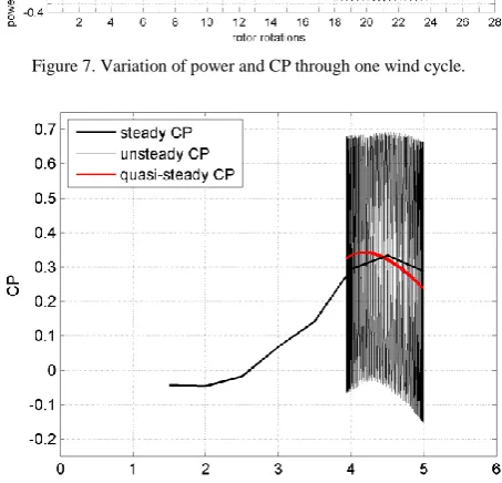
characteristic frequency equal to three times the rotor frequency would result in huge fluctuations in the rotor power PB. The variation of PB is shown in Figure 7 together with the fluctuating wind power Pw. As expected, the peaks of PB follow the wind variation much like the TB does. Maximum PB is 140Watts generated as Pw maximizes at the end of the 7th rotation, with magnitude of 207W. Also presented are the unsteady CP and quasi–steady CP using moving average smoothing. Smoothing the unsteady CP provides a useful comparative plot to the experimental data where the unsteadiness of the experimental CP over one rotor cycle is not captured. In addition, this is shown to be consistent with the cycle averaged method of computing for the rotor CP in steady wind conditions, that filters out the fluctuating nature of the blade torque to give a single value prediction of VAWT performance.
[image:4.595.314.541.148.366.2]Figure 5. Variation of U∞, λ, and α.
Figure 6. Variation of Tb and TB.
[image:4.595.57.284.248.734.2]Figure 7. Variation of power and CP through one wind cycle.
Figure 8. Performance of the VAWT in 12% fluctuating free stream.
In Figure 8, the plots of the unsteady CP and quasi– steady CP versus λ are shown relative to the steady wind performance at 7m/s. The fluctuations in the unsteady CP over the band of operating λ show a massively varying VAWT performance that greatly exceeds the limits of the steady wind CP. The maximum CP is recorded at 0.69 and occurs just after the 15th rotation (λ = 4.55). The minimum CP is seen to take place after the 21st rotation with a value of –0.15 (λ = 5). The wind cycle–averaged CP is computed to be 0.33 (λmean = 4.4) and is equal to the maximum steady wind CP of 0.33 at λ = 4.5. It is clear from the figure that the quasi–steady CP crosses the steady CP curve. Increasing wind speeds cause the CP to deviate from the steady CP curve and rise to higher levels as the λ falls to lower values. On the other hand, decreasing wind speeds cause the CP to drop below the steady CP curve as the λ rises. There is no discernible hysteresis in the quasi–steady CP curve.
[image:4.595.59.284.255.491.2] [image:4.595.55.285.497.734.2]a.
[image:5.595.55.284.49.331.2]b. c.
Figure 9. Lift coefficient loops for the reference case: a) full plot of cycles, b) zoom view of upwind loops, c) zoom view of downwind loops.
a.
b. c.
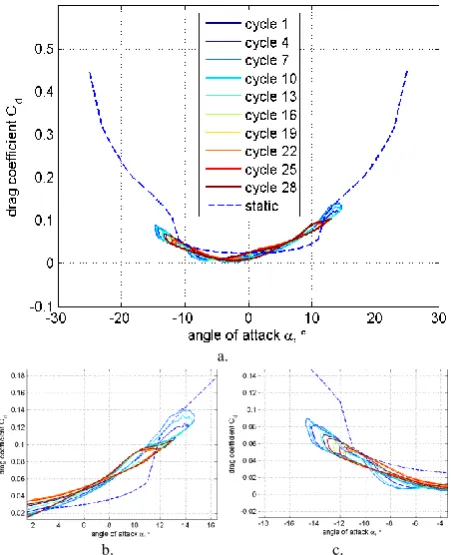
Figure 10. Drag coefficient loops for the reference case: a) full plot of cycles, b) zoom view of upwind loops, c) zoom view of downwind loops.
The drag coefficient loops for selected cycles are shown in Figure 10. It can be seen that all cycles exceed the static stall drag in the upwind (Figure 10b) with maximum Cd = 0.14 generated during the 7th rotor cycle. The trends of the Cd loops seem to follow the Cd line of the stalled condition for static aerofoil indicating that not only increases in lift are observed, but also in drag. Downwind drag does not follow the same trend. Maximum Cd of 0.09 is still generated in the 7th rotor cycle (Figure 10c). However, all rotor cycles have
their Cd loops follow the Cd line of the un–stalled condition for a static aerofoil. Although maximum Cl is at the 7th cycle, this is counteracted by the Cd, which is also at its maximum. Hence, the quasi–steady CP is not at its peak when U∞ is at the highest value. In fact, maximum quasi– steady CP is seen to occur at the 3rd and 12th cycles, when maximum Cd is 15% lower than the 7
th
cycle maximum of 0.14 while maximum Cl is only 2% lower than the 7th cycle maximum of 0.94.
VI. CONCLUSIONS
Numerical simulations using RANS–based CFD have been utilised to carry out investigations on the effects of steady and unsteady wind in the performance of a wind tunnel VAWT. Using a validated CFD model, steady wind simulations at U∞ = 7m/s were conducted and results have shown a typical performance curve prediction for this particular VAWT scale. Within the low λ range, there is a distinct negative trough, with drag–dominated performance consistent to experimental results. Minimum CP is computed to be –0.04 at λ = 2 and positive CP is predicted to be attained at λ’s higher than 2.5. Maximum CP is 0.33 at λ* = 4.5 and a shift in the CFD–predicted CP curve to higher λ’s is observed relative to the experimental CP profile.
Unsteady wind simulations revealed a fundamental relationship between instantaneous VAWT CP and Reynolds number. Following the dependency of CP to Reynolds number from experimental data, CFD data shows a CP variation in unsteady wind that cuts across the steady CP curve as wind speed fluctuates. A reference case with Umean = 7m/s, Uamp = ±12%, fc = 0.5Hz and λmean = 4.4 has shown a wind cycle mean CP of 0.33 that equals the maximum steady wind CP at λ = 4.5. Lift coefficient loops uncover performance characteristics of a blade at different points in the wind cycle that depict the presence of dynamic stall as lift values consistently exceed static stall lift in the upwind region. However, CP–λ loops do not show any hysteresis due to the quasi–steady effect of the very slow fluctuating wind relative to VAWT ω. Increasing wind speeds have more effect on the tangential component of lift than on drag, which helps improve the performance of the VAWT. Decreasing wind speeds limit the perceived α seen by the blades to near static stall thus reducing the positive effect of dynamic stall on lift generation.
NOMENCLATURE
c blade chord Cd drag coefficient Cl lift coefficient CP power coefficient
fc characteristic frequency of unsteady wind PB blade power (three blades)
Pw wind power
Tb blade torque (single blade) TB blade torque (three blades) Tu turbulence intensity U∞ free stream wind speed
Uamp amplitude of fluctuation of unsteady wind Umean mean speed of unsteady wind
[image:5.595.57.283.366.644.2]α angle of attack Δt time step size θ azimuth position λ tip speed ratio, Rω/U∞ λ* tip speed ratio at peak CP
λmean tip speed ratio corresponding to ωmean μ laminar viscosity
μt turbulent viscosity ω rotor angular speed
ωmean in unsteady wind, mean of ω CFD Computational Fluid Dynamics PIV Particle Image Velocimetry VAWT vertical axis wind turbine
REFERENCES
[1] "Climate Change 2007: The Physical Science Basis," Technical Report No. AR4, Intergovernmental Panel on Climate Change, Cambridge, United Kingdom and New York, NY, USA.
[2] Department of Energy Change and Climate. Renewable Energy in 2011, June 2012, Accessed online 31 August 2012, http://www.decc.gov.uk.
[3] Mcintosh, S. C., Babinsky, H., and Bertenyi, T., 2007, "Optimizing the Energy Output of Vertical Axis Wind Turbines for Fluctuating Wind Conditions," 45th AIAA Aerospace Sciences Meeting and Exhibit, Reno, Nevada.
[4] Mcintosh, S. C., Babinsky, H., and Bertenyi, T., 2008, "Unsteady Power Output of Vertical Axis Wind Turbines Operating within a Fluctuating Free-Stream," 46th AIAA Aerospace Sciences Meeting and Exhibit, Reno, Nevada.
[5] Danao, L. A., and Howell, R., 2012, "Effects on the Performance of Vertical Axis Wind Turbines with Unsteady Wind Inflow: A Numerical Study," 50th AIAA Aerospace Sciences Meeting including the New Horizons Forum and Aerospace Exposition, Nashville, TN, USA.
[6] Scheurich, F., and Brown, R. E., 2012, "Modelling the Aerodynamics of Vertical-Axis Wind Turbines in Unsteady Wind Conditions," Wind Energy, pp. 17.
[7] Ansys Inc. Fluent 13.0 Documentation, 2010.
[8] Amet, E., Maitre, T., Pellone, C., and Achard, J. L., 2009, "2d Numerical Simulations of Blade-Vortex Interaction in a Darrieus Turbine," Journal of Fluids Engineering, 131(11), pp. 111103-15.
[9] Consul, C. A., Willden, R. H. J., Ferrer, E., and Mcculloch, M. D., 2009, "Influence of Solidity on the Performance of a Cross-Flow Turbine " Proceedings of the 8th European Wave and Tidal Energy Conference., Uppsala, Sweden.
[10] Edwards, J., Durrani, N., Howell, R., and Qin, N., 2007, "Wind Tunnel and Numerical Study of a Small Vertical Axis Wind Turbine," 45th AIAA Aerospace Sciences Meeting and Exhibit, Reno, Nevada, USA
[11] Edwards, J. M., Danao, L. A., and Howell, R. J., 2012, "Novel Experimental Power Curve Determination and Computational Methods for the Performance Analysis of Vertical Axis Wind Turbines," Journal of Solar Energy Engineering, 134(3), pp. 11. [12] Hamada, K., Smith, T. C., Durrani, N., Qin, N., and Howell, R.,
2008, "Unsteady Flow Simulation and Dynamic Stall around Vertical Axis Wind Turbine Blades," 46th AIAA Aerospaces Sciences Meeting and Exhibit, Reno, Nevada, USA
[13] Howell, R., Qin, N., Edwards, J., and Durrani, N., February 2010, "Wind Tunnel and Numerical Study of a Small Vertical Axis Wind Turbine," Renewable Energy, 35(2), pp. 412-422.
[14] Mclaren, K., Tullis, S., and Ziada, S., 2011, "Computational Fluid Dynamics Simulation of the Aerodynamics of a High Solidity, Small-Scale Vertical Axis Wind Turbine," Wind Energy, 15(3), pp. 349-361.
[15] Raciti Castelli, M., Ardizzon, G., Battisti, L., Benini, E., and Pavesi, G., 2010, "Modeling Strategy and Numerical Validation for a Darrieus Vertical Axis Micro-Wind Turbine," ASME Conference Proceedings, 2010(44441), pp. 409-418.
[16] Raciti Castelli, M., Englaro, A., and Benini, E., 2011, "The Darrieus Wind Turbine: Proposal for a New Performance Prediction Model Based on Cfd," Energy, 36(8), pp. 4919-4934.
[17] Simão Ferreira, C. J., Bijl, H., Van Bussel, G., and Van Kuik, G., 2007, "Simulating Dynamic Stall in a 2d Vawt: Modeling Strategy, Verification and Validation with Particle Image Velocimetry Data," Journal of Physics: Conference Series, 75(1), pp. 012023.
[18] Simão Ferreira, C. J., Van Brussel, G. J. W., and Van Kuik, G., 2007, "2d Cfd Simulation of Dynamic Stall on a Vertical Axis Wind Turbine: Verification and Validation with Piv Measurements," 45th AIAA Aerospace Sciences Meeting and Exhibit, Reno, Nevada. [19] Tullis, S., Fiedler, A., Mclaren, K., and Ziada, S., 2008,
"Medium-Solidity Vertical Axis Wind Turbines for Use in Urban Environments," 7th World Wind Energy Conference, St. Lawrence College, Kingston, Ontario.