Speed Control of DC Servo Motor using Different Controllers

Speed Control of DC Servo Motor using Different

Controllers

V. Rangavalli1, K. Lavanya2. 1, 2

Department of Electrical and Electronics engineering, ANITS

Abstract: DC servo motor is widely used in many applications likeRobotics, ConveyorBelts and Camera. In this paper a dc servo motor using MATLAB has been designed whose speed may be investigated using conventional controllers and FUZZY, SMC, ANFIS controllers are applied to control the speed of servomotor, that gives better response, when compared to conventional controllers. In this paper a comparison among fuzzy logic controller, sliding model controller, Adaptive Neuro-Fuzzy Inference System (ANFIS) through MATLAB/Simulink software have been presented.

Keywords: FUZZY, SMC, ANFIS

I. INTRODUCTION

An electrical motor controlled with the help of servo mechanism. If the motor as controlled device, associated with servo mechanism is dc motor, then it is commonly known as DC servo motor. If the controlled motor is operated by AC it is called AC servomotor. Mechanical motion control systems finds widespread applications in industry since the invention of steam engine in eighteenth century. Since then the evolution of motion control has been rapidly influenced by development of electrical machines.A servo system mainly consists of three basic components - a controlled device, a output sensor, a feedback system. This is an automatic closed loop control system. Here instead of controlling a device by applying the variable input signal, the device is controlled by a feedback signal generated by comparing output signal and reference input signal. When reference input signal or command signal is applied to the system, it is compared with output reference signal of the system produced by output sensor, and a third signal produced by a feedback system. This third signal acts as an input signal of controlled device.This input signal to the device presents as long as there is a logical difference between reference input signal and the output signal of the system. After the device achieves its desired output, there will be no longer the logical difference between reference input signal and reference output signal of the system. Then, the third signal produced by comparing theses above said signals will not remain enough to operate the device further and to produce a further output of the system until the next reference input signal or command signal is applied to the system. Hence, the primary task of a servomechanism is to maintain the output of a system at the desired value in the presence of disturbances.

II. MODELING OF DC SERVO MOTOR

Direct current motors are widely used for industrial and domestic applications. The control of the speed of a DC motor with high accuracy is required. There are various DC motor types. Depending on type, a DC motor may be controlled by varying the input voltage or by changing the input current. In this paper, the DC servo motor model is chosen due to its good electrical and mechanical performances compared to other DC motor models. The separately excited DC motor is driven by applied armature voltage

Figure1.Block diagram of dc servo motor

T or =Torque developed by motor

B=equivalent viscous friction co-efficient of motor and load referred to motor J= equivalent moment of inertia of motor and load referred to motor

R or =armature resistance L or =armature inductance

or =armature voltage =armature current

The dynamics of a separately excited DC motor may be expressed as: The air gap flux ∅ is proportional to the field current

∅ = (1)

Torque developed by motor is proportional to the field current and air gap flux =

In armature controlled dc motor field current is kept constant. = (2)

The motor back emf being proportional to speed = (3)

The differential equation of armature current is

+ + = (4)

The torque equation is given by

J +B = = (5)

on taking Laplace transforms on both sides with zero initial conditions we get (s)= sω (s) (6)

(Ls+R) (s)+ (s) = (s) (7) (J +Bs)ω(s) = (s) (8)

The transfer function of the system is given by G(s) = ( ) ( ) (Ls+R) (s)+ (s) = (s)

(Ls+R) (s)+ sω(s) = (s)

( + ) ( ) + ∗(

( )) (s) = (s) (Ls + R) + (

( )) (s)= (s)

G(s) = _{( )} ( ) = _{( )} ( )* _{( )} ( )

Therefore the transfer function of motor is given by

G(s) =

( [( ) ( ) ] )

The armature circuit inductance is generally negligible i.e. L=0

( )

( ) =G(s) = ( [( )( ) ] )

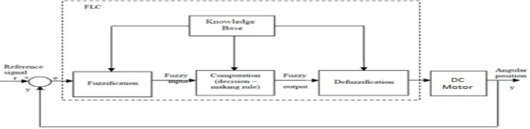
III. FUZZY LOGIC CONTROLLER

Fuzzy logic has currently used in control theory, artificial intelligence systems specially to control complex aircraft engines and control surfaces, helicopter control, missile guidance, automatic transmission, wheel slip control, auto focus cameras and washing machines ,railway engines for smoother drive and fuel consumption and many industrial processes.

The flc system usually done in four steps.

1) Fuzzification of the inputs

2) Rule evaluation.

3) Aggregation of the rules.

4) Defuzzification.

CE NL NM NS Z PS PM PL

NL NL NL NL NM NS NS Z

NM NL NL NM NS NS Z PS

NS NL NM NS NS Z PS PM

Z NM NM NS Z PS PM PM

PS NM NS Z PS PS PM PL

PM NS Z PS PS PM PL PL

PL Z PS PS PM PL PL PL

Table 1.Fuzzy rules table

IV. SMC CONTROLLER DESIGN

A. Sliding Mode Control Introduction

It is well known, that the sliding mode control is a popular robust control Method. However it has a reaching phase problem and an input chattering problem (as discussed above). These problems cause the sliding mode control (SMC) is very conservative to be used with other controller design methods because the state trajectory of the sliding mode control system is determined by sliding mode dynamics, which cannot have the same order dynamics of the original system. This leads to the introduction of robust controller design with novel sliding surface. To overcome the conservatism of the SMC, the novel sliding surface has been used which the same dynamics of the nominal original system has controlled by a nominal controller. The reaching phase problem can be eliminated, by using an initial virtual state that makes the initial sliding function equal to zero. Therefore, it is possible to use the SMC technique with various types of controller.

A linear system can be described in the state space as follows:

= ̇ Ax+Bu (1) Where ∈ , u ∈ R, A∈ Rn*n,and B∈ Rn and B is full rank matrix. A and B are controllable matrixes. The functions of state variables are known as switching function:

=sx (2) The main idea in sliding mode control is

1) Designing the switching function so that





0

2) Finding a controller ensuring sliding mode of the system occurs in finite time First of all, the system should be converted to its regular form:

̅ =Tx (3) T is the matrix that brings the system to its regular form

̇ = + (4)

̇= + + (5)

The switching function in regular form is: = +

On the sliding mode manifold ( = 0):

0= +

= - (6) From (6)&(4)

̇ = ( - ) (7) One of matrixes in product: should be chosen arbitrary. Usually (8) is used to ensure that is invertible

=

(8) can be calculated by assigning the Eigen value of (7) by pole placement method. Hence, switching function will be obtained as follows:

S= [ s s ]T (9) The control rule is:

= + (10) Where and are continuous and discrete parts, respectively and can be calculated as follows:

= -

A

x

A

= - sgn - (12) Where sgn is sign function. , and are constants calculated regarding to lyapunov stability function.

B. Modelling of DC Motor

The state space model of DC motor is as follows

The modelling and state space model of dc motor is already discussed in chapter2

̇ =Ax+Bu = −

− − +

0

(13)

In this equation x is two dimensional vector x = Where

= angular velocity of shaft. = armature current. u = the armature voltage. R= resistance of armature coil. L= inductance of the armature coil. = velocity constant.

= torque constant. J= moment of inertia.

b = viscous friction coefficient

By using the Laplace transform of (13), the transfer functions of system according to angular speed of shaft ( (s) ) and armature voltage (U(s)) can be calculated:

Take ̇(s)= (s) and ( )=U(s) from motor model we have

( )

( )= ([( ) ( ) ] ) (14)

( )

( )= ( )

( )

( )= ( ) (15)

(15) in time domain is as follows:

s (s)+ + s (s)+( ) (s)= U(s) + + +( ) = u

(16)

̇= ̇= (a) From eqn (16)

̇+ + +( ) = u

̇ =-( + ) -( ) + u (b)

Therefore the state space model is

̇_̇ = 0 1 +

0

(17)

= - ( ) (18)

= -( + ) (19)

C. Design Of The Switching Function

We are going to set the angular velocity over a certain value r, so switching function is = ( -r) + (20)

If the controller switching function is designed to be placed on the surface = 0. Put = 0 in eqn (20) 0= ( -r) +

We have = and = ̇= ̇

- r+ =0

= (r- )

( )= On applying integration on both sides from 0 to t as limits ∫

( )=∫ It gives log(r− )= - t

(r− )= From above equation

= r- (21)

̇= (22)

=

= (23)

= - (24)

As (21), (22) and (24) shown determines the speed of convergence of the system output So it is better to choose a small negative value Thus, the switching function was designed as follows

= ( -r) + We have = -

=− ( -r) +

σ = (- ( − ))+ ̇) (25)

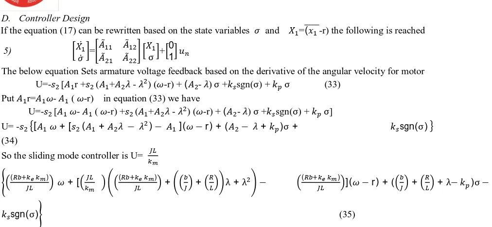
D. Controller Design

If the equation (17) can be rewritten based on the state variables and =( -r) the following is reached

5) ̇

̇ = σ +

0

1

The below equation Sets armature voltage feedback based on the derivative of the angular velocity for motor U=- [ r + ( + - ) ( -r) + ( - )σ + sgn(σ) + σ (33)

Put r= - ( -r) in equation (33) we have

U=- [ - ( -r) + ( + - ) ( -r) + ( - )σ + sgn(σ) + σ]

U= - [ + [ ( + − )− ]( −r) + ( − + )σ+ sgn(σ) (34)

So the sliding mode controller is U=

( )

+ [ ( ) + + λ+λ − ( ) ]( −r) + ( + +λ− )σ −

sgn(σ) (35)

Is controller designed for controlling the speed of dc motor now consider the real model switching function and controller design for the same motor is given by solving The controller u is given by U=1/174.5((33.97 e(t))-(c-30.8)e(t)+k sign(s)

V. ARTIFICIAL NEURAL NETWORKS

Artificial Neural Networks or ANN’s is a very powerful technique for solving complex dynamic systems.

A. Types of Neural Network

1) Single Layer Feed-forward Network

2) Multi layer feed-forward network

3) Recurrent network

B. Mathematical Modeling Of An ANN

Artificial neurons have almost the same structure as the biological neurons, but with different names and added elements. An ANN mimics the function of a biological neural network and hence it is considered as a very powerful tool that a control engineer can use to solve difficult non-linear problems. The ANN architecture consists of multiple neurons connected together; each neuron has a similar structure to other neurons (Fukushima Kunihiko, 1975). Figure 4.5 shows a single artificial neuron.

Figure 3. Artificial neuron structure

Each neuron consists of input , weight , bias _, transfer function _ and the output a. The output of the neuron a can be written in terms of the other elements as

The network input can be written as

Figure 4. Multi input neuron

The interconnections of single neurons to other neurons form the architecture of the neural network. The interconnection of multiple single neurons to form an ANN is shown in figure 4.7

Figure 5. Neural network structure

As mentioned before, ANN’s are very powerful tools to solve complex problems and therefore complex control systems. They have a parallel structure that makes them capable to accept large data and process it at one time; which will reduce the time needed for the whole control process to be done. One other important advantage of ANN’s is that they are capable to “generalize”, which makes them act as a smart controller, this means that the controller is able to deal with new type of input data, this means that the controller has not been trained with that type of data and is let by itself to decide how to deal with any change in the non-linear parameters to reduce their effect. Although, many controllers have been implemented for servomotors, they are not efficient enough in some cases, especially when the servomotor used in a critical application requires a high efficient motor.

VI. ANFIS CONTROLLER

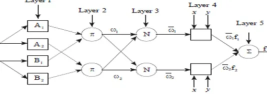
A typical architecture of an ANFIS is shown in Figure , in which a circle indicates a fixed node, whereas a square indicates an adaptive node. For simplicity, we consider two inputs x, y and one output z. Among many FIS models, the Sugeno fuzzy model is the most widely applied one for its high interpretability and computational efficiency, and built-inoptimal and adaptive techniques. For a first order Sugeno fuzzy model, a common rule set w1ith two fuzzy if–then rules can be expressed as:

Rule 1: if x is A1 and y is B1 , then z11 = p x + q y + r

Rule 2: if x is A2 and y is B2 , then z 22= p x + q y + r

where Ai and Bi are the fuzzy sets in the antecedent, and pi, qi and ri are the design arameters that are determined during the training process. As in Figure 2, the ANFIS consists of 3layers

1) Layer 1: Every node i in the first layer employ a node function given by:

where μAi and μBi can adopt any fuzzy membership function (MF).

The number of epochs was 100 for training. The number of MFs for the input variables e and de is 7 and 7, respectively. The number of rules is then49 (7×7 = 49). The triangular MF is used for two input variables. It is clear from that the triangular MF is specified by two parameters. The training and testing root mean square (RMS) errors obtained from the ANFIS. The section presents a methodology for developing adaptive speed controllers in a DC servo motor drive system.

A PI controller is employed In order ANFIS info:

Number of nodes: 21, Number of linear parameters: 12, Number of nonlinear parameters: 8 Total number of parameters: 20

Number of training data pairs: 59 Number of checking data pairs: 55 Number of fuzzy rules: 4

Start training ANFIS

a) 0.00134332

b) 0.00133966

VII. SIMULATION AND RESULTS

A. Simulation Diagrams And Results Of Dc Servo Motor With FUZZY, SMC, ANFIS

Figure6. Simulation Diagram of DC servo motor using Fuzzy logic controller

Figure7. Simulation Diagram of DC servo motor using Sliding mode controller

Figure9.Simulation output of Fuzzy logic controller for dc servo motor

Specifications are tr = 2.5 sec, ts = 4 sec %MP = 0

Figure10.Simulation output of Sliding mode controller for dc servo motor

Specifications are tr = 0.25 sec,ts = 0.5 sec, %MP = 0

Figure11.Simulation output of ANFIS controller for dc servo motor

Specifications are tr = 0.3 sec,ts = 0.4 sec, %MP = 0

VIII.CONCLUSION

REFERENCES

[1] E.H. Mamdani, “Application of Fuzzy Algorithm for Control of Simple Dynamic Plant”, Proc. IEE121 (12), pp.1585-1588, 1974.

[2] Hans Butler, Ger Honderd, Job Van Amergoen, “ Model Reference Adaptive Control of a Direct – Drive DC motor”, IEEE Control System Magazine, pp. 80-84

[3] Gopal K. Dubey, “Fundamental of electrical Drives", Narosa Publication 2009.

[4] Mustafa Aboelhassan, “Speed Control of D.C. Motor using Combined Armature and Field Control,” Doctoral Degree Programme (2), FEEC BUT. [5] Michael, P., 2008," Computer Simulation of Power Electronics and Motor Drives", Lubbock, Texas Tech University, USA

[6] Khuntia, K.B. Mohanty, S. Panda and C. Ardil, “A Comparative Study of P-I, I-P, Fuzzy and Neuro-Fuzzy Controllers for Speed Control of DC Motor Drive”, International Journal of Electrical and Computer

[7] M.M. Shaker,Y.M.B.I.Al-khashab, “Design and implementation of fuzzy logic system for DC motor speed control”, first International Conference on Energy, Power and Control, pp.123-130, 2010.

[8] K.M.A.Prasad, B.M. Krishna, U. Nair, “Modified chattering free sliding mode control of DC motor”, international journal of modern engineering research, vol. 3, pp.1419-1423, 2013.

[9] I. H. Altas and A .M. Sharaf, “A Generalized Direct Approach for Designing Fuzzy Logic Controllers in Matlab/Simulink GUI Environment”, International Journal of Information Technology and Intelligent Computing, Int.J. IT&IC no.4 vol.1, 2007

[10] Auzani bin jidin”Sliding mode Variable structure control design principles and application to dc drives” Universiti Teknologi Malaysia,OCTOBER 2004

AUTHOR’S BIOGRAPHY

Rangavalli Vasa Received her Master degree in 2012 in Control systems at Anits, Visakhapatnam, India, and Bachelor degree in 2007 in Electrical & Electronics Engineering from SVP Eng.college, P.M Palem, and India. She is Pursuing Ph.D in the area of Power Systems at JNTUK. She is currently working as an Assistant Professor of Electrical and Electronics Engineering Department at ANITS, Visakhapatnam, India.

Mail id: [email protected]

Lavanya Komma Received her Master degree in 2010 in Power Electronic from JNTU University (AURORA Eng College), Hyderabad, India, and Bachelor degree in 2005 in Electrical & Electronics Engineering from TPIST, Bobbili, India. She is Pursuing Ph.D in the area of Power Electronics and Drives at JNTUK.She had 10 years teaching experience. She is currently working as an Assistant Professor of Electrical and Electronics Engineering Department at ANITS, Visakhapatnam, India.