Neural Network in Detecting the Attribute of Faults in 3 D Seismic Interpretation

Neural Network in Detecting the Attribute of Faults

in 3-D Seismic Interpretation

Tomiwa A. C.

Physics and Electronics Department, Adekunle Ajasin University Akungba Akoko, Ondo State, Nigeria akinyemi.tomiwa@aaua.edu.ng

Abstract: Neural network had become rapidly apparent that despite being very useful in some domains, it failed to capture certain key aspects of human intelligence. According to one line of speculation, this was due to their failure to mimic the underlying structure of the brain. In order to reproduce intelligence, it would be necessary to build systems with a similar architecture. When a neuron in the brain is activated, it fires an electrochemical signal along the axon. This signal crosses the synapses to other neurons, which may in turn fire. A neuron fires only if the total signal received at the cell body from the dendrites exceeds a certain level (the firing threshold). The result shows that within offset 6ms in the horizon have distorted amplitude repeatedly for the three wavelets, which is mapped out in the model to be fault line. This means within the horizon, fault (f) has been detected which is a major hydrocarbon indicator that can be interpreted using 3D tools. The second horizon also shows a synclinal structure which is an indication of the existence of a fault line ( ) in the lower bed of the horizon. These two lines can be interpreted to be hydrocarbon container within this region as a closure which is a structural trap.

Key words: Horizon, Structural Trap, Fault, anticlines and synclines

I. INTRODUCTION

Neural networks grew out of research in Artificial Intelligence; specifically, attempts to mimic the fault-tolerance and capacity to learn of biological neural systems by modeling the low-level structure of the brain (Patterson, 1996: 3-10). The main branch of Artificial Intelligence research in the 1960s -1980s produced Expert Systems. These are based upon a high-level model of reasoning processes (specifically, the concept that our reasoning processes are built upon manipulation of symbols). The brain is principally composed of a very large number (circa 10,000,000,000) of neurons, massively interconnected (with an average of several thousand interconnects per neuron, although this varies enormously). Each neuron is a specialized cell which can propagate an electrochemical signal. The neuron has a branching input structure (the dendrites), a cell body, and a branching output structure (the axon). The axons of one cell connect to the dendrites of another via a synapse. The strength of the signal received by a neuron (and therefore its chances of firing) critically depends on the efficacy of the synapses. Each synapse actually contains a gap, with neurotransmitter chemicals poised to transmit a signal across the gap. One of the most influential researchers into neurological systems (Donald Hebb) postulated that learning consisted principally in altering the "strength" of synaptic connections. For example, in the classic Pavlovian conditioning experiment, where a bell is rung just before dinner is delivered to a dog, the dog rapidly learns to associate the ringing of a bell with the eating of food. The synaptic connections between the appropriate part of the auditory cortex and the salivation glands are strengthened, so that when the auditory cortex is stimulated by the sound of the bell the dog starts to salivate. Recent research in cognitive science, in particular in the area of non-conscious information processing, have further demonstrated the enormous capacity of the human mind to infer ("learn") simple input-output co-variations from extremely complex stimuli. To recognize a pattern, one can use the standard multi-layer perception with a back-propagation learning algorithm or simpler models such as self-organizing networks (Kohonen, 1997) or fuzzy c-means techniques (Bezdek, 1981; Jang and Gulley, 1995). Self-organizing networks and fuzzy c-means techniques can easily learn to recognize the topology, patterns, or seismic objects and their distribution in a specific set of information. Much of the early applications of pattern recognition in the oil industry were highlighted in Aminzadeh (1989a). An usual though sophisticated form of structural modeling under earthquake loading is the iterative integration of the set of differential equations which establish equilibrium under dynamic conditions, usually referred to as equation of motion (eq1)

Müt + ůt + ut = Pt 1

In which ü(t), ů(t) and u(t) are respectively the vectors of nodal acceleration, velocity and displacement at instant t; M denotes the

There are two basic approaches to solution of equation of dynamic equilibrium of eq1 as viz;

In order to use direct integration of equation 1, it is necessary to subdivide the time domain in a number of finite intervals of duration t. Equation 1 develops, hence to the following form:

Mü +Ců + Ku = P 2

The integration of the above system of equation may be attempted by explicit or implicit methods as discussed by Clough and Penzien 1993.

If an explicit method is adopted, the response at time may be defined by establishing equilibrium at time i.e , equation 2 needs to be solved once per step.

If contrarily, implicit method is to be used then it is necessary to define a rule of variation for the acceleration, and therefore, velocity and displacement in each time step. Consequently, the solution at the time depends on the values of ü(t), ů(t) and u(t),

but also depends on the contemporaneous values at time . it is therefore likely that equation 2 needs to be solved iteratively until adopted values of acceleration enables equilibrium. If the earthquake to which the structural model is to be analyzed is presented by a ground motion record, such as the one of figure 1 the chosen time step (usually constant) for the iterative resolution of the system of equation 2 implies that the accelerogram be defined by a finite steps of acceleration. The system of equation can then be solved in order to satisfy the prescribed conditions for dynamic equilibrium for every time interval under consideration, once for explicit method or more than once for implicit ones.

II. MODELLING ARTIFICIAL NEURAL NETWORK AND SYSTEM MODIFICATION

In a bid to understand modeling of neural networks, it is worth noting that reference is made to the biological system from which it evolved and a concise mathematical model will do just fine.

A. The Biological Model

Artificial neural networks born after McCulloc and Pitts introduced a set of simplified neurons in 1943. These neurons were represented as models of biological networks into conceptual components for circuits that could perform computational tasks. The basic model of the artificial neuron is founded upon the functionality of the biological neuron. By definition, “Neurons are basic signaling units of the nervous system of a living being in which each neuron is a discrete cell whose several processes are from its cell body”

Figure 1: Biological Neuron

The biological neuron has four main regions to its structure. The cell body, or soma, has two offshoots from it. The dendrites and the axon end in pre-synaptic terminals. The cell body is the heart of the cell. It contains the nucleolus and maintains protein synthesis. A neuron has many dendrites, which look like a tree structure, receives signals from other neurons. A single neuron usually has one axon, which expands off from a part of the cell body. This I called the axon hillock. The axon main purpose is to conduct electrical signals generated at the axon hillock down its length. These signals are called action potentials.

B. The Mathematical Model

number, and represents the synapse. A negative weight reflects an inhibitory connection, while positive values designate excitatory connections. The following components of the model represent the actual activity of the neuron cell. All inputs are summed altogether and modified by the weights. This activity is referred as a linear combination. Finally, an activation function controls the amplitude of the output. For example, an acceptable range of output is usually between 0 and 1, or it could be -1 and 1. Mathematically, this process is described in the figure 2 below:

Figure 2: Mathematical Model of Biological Neuron

From this model the interval activity of the neuron can be shown to be:

The output of the neuron, , would therefore be the outcome of some activation function on the value of .

C. Buckingham Pi Theorem

In attempting to solve a problem, an engineer often tries analytic mathematics methods first. Equations stating the relations that must be satisfied are set up. The Buckingham pi theorem is a very powerful tool of dimensional analysis. This theorem is particularly well adapted for use by engineers since little mathematical knowledge is necessary. The underlying physical principles, however, must be well known. This theorem was formulated by Dr. Edgar Buckingham of the Bureau of Standards. Initially dimensions are analyzed using Rayleigh’s Method. Alternatively, the relationship between the variables can be obtained through a

method called Buckingham’s π. Buckingham’s pi theorem states that: If there are n variables in a problem and these variables contain m primary dimensions (for example M, L, T) the equation relating all the variables will have (n-m) dimensionless groups.

Buckingham referred to these groups as π groups. The final equation obtained is in the form of: π = f (π , π , ….. π ) NOTE:

The π groups must be independent of each other and no one group should be formed by multiplying together powers of other

values of the indices (the exponent values of the variables). In this method of solving the equation, there are 2 conditions: Each of the fundamental dimensions must appear in at least one of the m variables

III. ENGINEERING APPLICATION OF BUCKINGHAM’S PI THEOREM.

As an introductory problem leading up to the theorem, consider the following very simple example:

Suppose it is desired to find the time t required for an object traveling at a constant velocity (v) to traverse a distance d. The relation t=d/v is unknown, and it is desired to solve the problem by analysis. A start is made by assuming (justification for this assumption will be given later) that the equation for t takes the following form: t= . Where C is a numerical constant and a, and b are unknown exponents. Since t has the dimension of time; d, that of length; and v, that of length divided by time, it is obvious that if the equation is to be dimensionally consistent, a must equal 1 and b must be -1. Hence t= C (d/v). The constant t may be evaluated rather easily in the laboratory by a single experiment, for example, by pulling a cart at constant velocity and measuring the time required to travel a given distance. Although the above example Is rather trivial, it illustrates one important point: a constant in an equation was evaluated by a single experiment. The equation thus formed, however, applies in all cases. The Buckingham pi theorem is basically just a refinement of the method used in this example. The pi theorem is somewhat more sophisticated and may be applied to more intricate problems. The Buckingham pi theorem state that if n quantities (force, viscosity, displacement, etc.) are concerned in a problem and if these n quantities are expressible in terms of m dimensionless groups which can be formed by combinations of the quantities. If the (n-m) groups are called P1, P2, P3, etc., then the solution of the problem must take the form: F (P1, P2, P3,…)=0. It will be noted that this equation can be solved for any particular pi. Some example illustrating the use of the pi theorem will be given. The symbol for a dimension will be taken as the capital of the first letter in the name of the dimension. Thus M is taken as the symbol for mass; L, for length; T, for time, etc. As the first example, consider the problem of a navel architect who wishes to plot the water resistance to motion of a ship versus the velocity of the ship. An analytical approach was tried but difficulties were encountered the pi theorem was restored to. The force of water resistance will in general depend upon the shape of the ship. However if consideration is limited to ships of similar shapes, then shape need no longer be considered. In this case some “characteristic linear dimension” should be specified to indicate relative size. Then the important qualities in concentration with this problem are:_{P = force on the ship = ML T}

S=immersed surface area = L

I=a liner dimension (to indicate relative size) = L

v(Nu)=kinematic viscosity of water =

V=velocity of the ship =L _T

ρ=density of the fluid = M _L

It will be seen that there are six quantities and three dimensions. Hence 6-3=3 pi’s are expected. The general expression for a pi takes the shapes:

π = P S I v V ρ

Substitution the dimensional equivalents:

π = (M L T⁄ )(L )(L)(L ⁄T )(L T⁄ )(M L⁄ )

If the pi is to be dimensionless, the exponent of M, N, and T must add up to zero separately. Whence:

a+f = 0 (For M)

a + 2b + c + e – 3f = 0(For L) -2a – d – e = 0 (For T)

There are six unknowns and three equations; hence, values may be arbitrarily assigned to three variables and the values of the other three variables determined from the above equations. Thus for choose a= 1, c= 0, e= 0. Inserting these values in the equations, one finds that f= -1, d= -2, b= 0.

=

For P2, choose a = 0, b = 0, e = 1. Solving the system of equations, one discovers that f= 0, c= 1, d= -1. = Since ⁄ is obviously a dimensionless quantity,

Then from the pi theorem: F ( _{, ,} ) = 0

If attention is restricted at present to ships which are similarly loaded (that is, each ship displaces relatively the same amount of water), then the ratio ⁄ will be the same for ships and may be omitted here.

Then F ( _, ) = 0; Solving for = F ( )

Now our naval architect could experiment on a model boat, varying the velocity of the model boat with respect to the fluid in which it floats and measuring the force upon the boat. Then if instead of merely plotting P versus V, he would plot ⁄ vertically against ⁄ horizontally, he would have a curve which, according to the pi theorem is m, applies to all ships. To find the curve of

P versus V for any ship, it is merely necessary to alter the coordinate of the above curve by the appropriate values of ρ, v, I. The

simplicity resulting from the use of the pi theorem is apparent from these results. A single curve shows the effect of five variables. If the data were treated in the more conventional manner, plotting P versus V as parameters, and if just five values of each parameter were considered, it would be necessary to plot 5 = 125 curves. It might be that the navel architect would wish data on just a few specific points instead of a complete curve In this case the analysis is somewhat simpler. Let primes refer to quantities connected with model boat, and let quantities without primes refer to the full-sized ship. Then

= F ( ) (1)

′

′ ′ = F ( ′ ′ ′) (2)

Now if the argument of the function f (that is, ⁄ ) is the same for both the model and the full sized ship, then f will have the same value in each case.

Hence if

( ) = ( ′ ′ _′) (3)

V’ = ( ′ ′⁄ ′)V

Then (1) divide by (2) :

P = ( ⁄ ′ ) P’ (4)

( ⁄ )( ′ ⁄ ′) = f( ⁄ )/f(I’V’/v’)

Hence if the model is given the velocity indicated by equation (3), then the force on the model and the real ship will be related by (4). Note that the mathematical manipulations used above are equivalent merely to equating the two pi’s for the model and for the full-sized ship. Now if the discussion is not limited to similarly loaded ships, then the quantity / will have different values for

different ships, and this quantity must be considered. In this case: = f ( , ) and it will be necessary to plot

versus for different values of as a parameter. The artificial neural networks which we describe in this course are all variations on the parallel distributed processing (PDP) idea. Then architecture of each network is base on very similar building blocks which perform the processing. In this section we first discuss these processing units and discuss different network topologies. Learning strategies as a basis for an adaptive system will be presented in the last section.

A. Networks With Threshold Activation Function

A single layer feed-forward network consists of one or more output neurons o: each of which is connected with a weighting factor

ἰ to all of the inputs i. In the simplest case the network has only two inputs and a single output. The input of the neuron is the

Y=F(∑ + )

The activation function F can be linear so that we have a linear network, or nonlinear. In this section we consider the threshold {or Heaviside or sgn} function.

( )= 1 > 0 −1 ℎ

The output of the network thus is either +1 or -1 depending on the output. The network can be used for classification task. It can be decided whether an input pattern belongs to one of the two classes. The separation between the two classes in this case is a straight line, given by the equation (5)

+ + θ = 0 (5)

The single layer network represents a linear discriminant function.

Equation (5) can be written as;

= − (6)

And we see that the weights determine the slope of the line and the bias determines the offset (i.e., how far the line is from the origin). Note that also the weights can be plotted in the input space: the weight vector is always perpendicular to the discriminant function.

+

+

o o + + +

o + +

o +

Figure 3: Geometric representation of the discriminant function and the weights.

IV. METHODOLOGY

Seismic waves either generated by earthquakes or artificial explosion near the Earth surface are considered to be sinusoidal waves of varying amplitudes depending on the characteristics of sub-surface in which they travel. In this work piece, the equation of wave that is used in modeling the neural network is of the form:

P(x, y, z, t) = Acos( t+ φ) (7)

Where ω = Angular Frequency in radians/second = 2π

= Frequency ( cycles/second or hertz) A= Amplitude of wave in metres(m)

Φ = phase in rad, φ = П

These terms completely characterize wave-fields in space-time, frequency-space, and frequency-wave-number. We can think of wave-field as actually being the sums of sinusoidal style waves having the general form of Equation 7, where A = A(x, y, z, ω = 2π ) is a positive amplitude as a function of spatial position (x, y, z) and frequency, and φ = φ(x, y, z, t) is the so called wavelet phase, it is worth noting that the network is trained such that negative amplitude is not classified, since any wave whose amplitude falls short of a specified positive value is classified as noise. The main point is that the wave-fields actually exist in three-dimensional space-time and can be characterized in many different ways. In this research, we will mostly be concerned with wave-fields measured on one surface. As any given sinusoid propagates through the Earth, its wavelength and amplitude change as functions of both reflection strength and sound speed. Although, these quantities can also change purely as a function of the material through which they are propagated.1

A. Analysis of Modeled Equation

To deploy a model, we apply the Buckingham’s PI theorem to equation 7. Writing the equation as a function we have:

F { ( , ), , , , }= 0 Number of variables, n = 5

Number of fundamental dimension, m = 3, i.e., [ ], [L], [T]. Number of dimensionless group = n-m = 5-3 = 2

Dimension of P(r, t) = [L] Dimension of A = [L] Dimension of = [T-1]

Dimension of t = [T]

Dimension of φ = [arcT]

The recurring sets of variable that are chosen are and φt. Such that: = [LT-2] ; therefore [L] = t2

φt = [TarcT]; therefore [T] = t

P(r, t) has a dimension of [L], therefore, P(r, t) [L-1] is dimensionless. Hence,

π1 = ( , ) _t

π2 = t

Thus, F (π1, π2) = 0 Model graph of π1 against π2 gives a generalization of the expected behavior of the design. If an engineer intends

to make an actual design, all he needs to do is to incorporate the true value of the variables, A, and t (for the desired machine), for all those chosen values of A, and t, what the engineer gets is a graph of maximum amplitude ( , ) against time t.

B. Conception And Programming

The programming language employed in modeling of the neural design is C codes, these codes are used to program Motorola microcontroller unit, with a 32-bits display screen .These are indicated in appendix ……..There is an interfacing port on the design to which a personal computer can be connected in order to have a detailed picture of the waveforms, the microcontroller has been coded to recognize the interfacing hardware. The neural has been trained and programmed to detect the fault line, this has been achieved in this research by drawing a line along the various distorted amplitude of the wavelets.

V. RESULTS DISCUSSION AND DATA ANALYSIS

TABLE 1: SIMULATED WAVELET I

t/ms A/m F/Hz φ/rad P (r, t)/m

3.0 28.3 21 0.39 20

6.0 63.8 18 0.33 34

12.0 40.0 14 0.26 10

15.0 12.2 11 0.20 4

18.0 7.5 21 0.39 -7

21.0 11.0 18 0.33 -10

24.0 2.0 18 0.33 -2

27.0 7.5 30 0.55 6

30.0 7.0 31 0.57 7

From the table above, the parameters used in describing the seismic wave can be analyzed below to reflect the modeling steps: Time, t (ms): this refers to the time of arrival of seismic waves at receiving equipment called geophone (a device regarded as an analog-to-digital converter). This has been preset to have a value of 3ms in this artificial neural network model. The travel time(t) may or may not have a constant interval as shown in the table above since travel times or arrival times of the seismic waves at geophones depends on specific attributes of sub-surfaces at which reflections occur.

Amplitude, A (m): this refers to the maximum displacement on seismic wave fronts. This has varying magnitudes at different times of travel due to the variation in the properties of layers in which they propagate. Maximum amplitude of 58.4m is observed at 9ms. It is expected that a peak will be seen at time of value 9ms.

Frequency, F (Hz): This is defined as the number of complete cycles seismic waves make in one second. These are randomly selected from computer generated numbers for this work. A maximum frequency of 31Hz is observed at time 30ms. The values of

frequencies selected are used to calculate magnitudes of wavelengths (λ) and phases (φ) with the aid of the following equations:

V = F λ (8)

Φ = П (9)

Phase, (φ): this refers to the offset of a seismic wavelet from a point o measured in radian (abbreviated as rad). It is given by equation 9 .Each value of phase is obtained by substituting the respective wavelengths into equation 9. For wavelet I, the phases of particles on the seismic wave are in the range 0.20≤ φ ≤ 0.57. represented by positive and negative numbers on the 5th column in Table 1. Actually, these are not supposed to be negative but the negative sign shows that the particles on the seismic wavelet I at these points are moving in the opposite directions with respect to those having positive displacements.

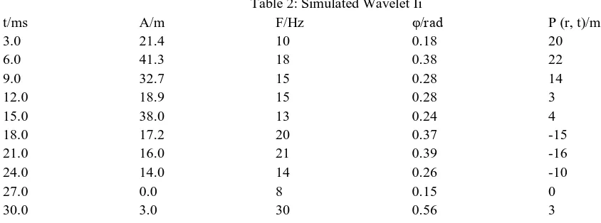
Table 2: Simulated Wavelet Ii

t/ms A/m F/Hz φ/rad P (r, t)/m

3.0 21.4 10 0.18 20

6.0 41.3 18 0.38 22

9.0 32.7 15 0.28 14

12.0 18.9 15 0.28 3

15.0 38.0 13 0.24 4

18.0 17.2 20 0.37 -15

21.0 16.0 21 0.39 -16

24.0 14.0 14 0.26 -10

27.0 0.0 8 0.15 0

30.0 3.0 30 0.56 3

41.3m is observed at 6ms, the frequencies are similarly computer generated and the phase is in the range 0.15 ≤ φ ≤ 0.56. Maximum

displacement of 22m is evident at the same 6ms arrival time that is characterized by a peak on the waveform below.

Table 3: Simulated Wavelet Iii

t/ms A/m F/Hz φ/rad P (r, t)/m

3.0 168.0 47 0.87 -31

6.0 0.0 45 0.83 0

9.0 36.2 18 0.33 8

12.0 2.0 23 0.42 -1

15.0 11.0 28 0.52 -11

18.0 27.0 30 0.55 -19

21.0 23.0 25 0.46 -19

24.0 18.0 22 0.41 -15

27.0 10.0 21 0.39 -7

30.0 2.6 36 0.67 1

Figure 4: The model displacement from the simulated wavelets.

Structural traps are formed as a result of changes in the structure of the subsurface due to processes such a folding and faulting, leading to the formation of domes, anticlines, synclines, and folds. Examples of this kind of trap are an anticline trap. They are more easily delineated and more prospective than their stratigraphic counterparts, with the majority of the world’s petroleum reserves being found in structural traps.

Fault Trap

Fold Trap

Figure 5: Monitoring and Detection of Fault

VI. CONCLUSION

Faults are lines of discontinuity which show an indication of an obstacle or a buried material. Faults can also be classified as traps. Since fault acts as petroleum traps and flow barriers, their identification and mapping is an important aspect of seismic interpretation. Supervised learning algorithm has been employed in the artificial neural network model which makes fault lines to be drawn across points of significantly prominent amplitude regarded as discontinuities. This forms an important section in this research because it is the main motive of this work (i.e fault mapping in 3-D seismic sections). Geostatistical distribution of porosity, permeability, thickness, texture, lithology and shale volume fraction of reservoir rocks are pertinent to fault detection by the designed artificial neural network model. Prior to fault detection is monitoring of displacement magnitudes on the seismic wavelets. The neural network trained in this project has detected two major faults within the horizons F1 and F2. From the fore-going analysis it can be concluded that Neural network is an effective tool for detecting and mapping geological features in 3-D seismic analysis. Also, to effectively map fault and other geological features like syncline, anticline, etc a neural network need to be trained to perform such a task. Hence, the artificial neural network generates output functions by observing clusters of changes in the input patterns.

REFERENCES

[1] Aminzadeh, F. and Chatterjee, s., (1984). Applications of clustering in Exploration Seismology. Geoexploration, 23: 147 – 159. Aminzadeh, F., (1989a).

Pattern Recognition and Image Processing. Elsevier Science, Amsterdam

[2] Aminzadeh, F. et al., (1994). Adaptive Neural Network For generation of artificial Earthquake precursors. IEEE Trans. Geosci. Remote sensing, 32(6)

[3] Baldwin, J.L. et al., (1990). Application of Neural Network to the Problem of Mineral Identification from Well Logs. Log Analysis, 3: 27

[4] Bezdek, J.C., (1981). Pattern Recognition with Fuzzy Objective Function Algorithm. Plenum Press, New York, N

[5] Boadu, F.K., (1997). Rock Properties and Seismic Attenuation:Neural Network Analysis. Pure Appl. Geophys., 149: 507-52

[6] Chawathe, A. et al., (1997). Interwell Property Mapping Using Crosswell Attributes. SPE 38747. SPE Annu. Tech. Conf. and Exhibition, San Antoni

[7] Clough, R.; Penzien, J. (1993) – Dynamics of Structures, McGraw-Hill International Editions, Singapor

[8] Hetch-Nielsen, R., (1989). Theory of Backpropagation Neural Networks. Presented at IEEE Proc., Int. Conf. Neural Network, Washington DC Jang, J.S.R. and

Gulley, N., (1995). Fuzzy Logic Toolbox. The Math works Inc.,Natick, M

[9] Klimentos, T. and McCann, C., (1990). Relationship among Compressional attenuation, porosity, Clay content and permeability in sandstone. Geophysics, 55:

99101 Kohonen, T.,(1997). Self-Organizing Maps, 2nd Edition. Springer, Berli

[10] M. Verleysen, D. Francois, G. Simon, and V. Wertz., (2003). On the Effects of Dimensionality on data analysis with Neural Networks. J. Mira (Ed.): IWANN

2003, LNCS 2687, pp. 105-112, 2003. Springer-Verlag Heidelberg 200

[11] Monsoon , G.D and Pita, J.A., (1997). Neural Network Prediction of pseudo-logs For net pay and Reservoir property Interpretation: Greater Zafiro field area,

Equatorial Guinea. SEG 1997 Meet., Dallas, TX.

[12] Nikravesh, M. and Aminzadeh, F., (2001). Mining and fusion of petroleum data with Fuzzy logic and Neural Network agents. J. Pet. Sci. Eng., 29:221-23

[13] Nikravesh, M.,(1998a). Mining and Fusion of Petroleum data with Fuzzy logic and Neural Network agents. CopyRight Report, LBNL-DOE, ORNL-DOE, and

[14] Nikravesh, M., (1998b). Neural Network Knowledge-based Modeling of rock properties based on well log databases. SPE 46206, 1998 SPE Western Reg. Meet., Bakersfield, CA, 10-13 Ma Nikravesh, M. et al., (1996). Model identification of Nonlinear time-variant Processe

[15] Nikravesh, M., and Aminzadeh, F.,. et al., (1998). Data mining and fusion with Integrated neuro-fuzzy agents. Rock properties and seismic attenuation.JCIS

1998. Fourth Joint Conf. on Information Sciences, NC, USA, October 23-28 Patterson, D (1996) Artificial Neural Networks. Singapore: Prentice Hall.

[16] Pezeshk, S., et al., (1996). Geophysical log interpretation using Neural Network. J. Comput. Civil Eng., 10: 13

[17] Rogers, S.J., Fang, J.H., Karr, C.L and Stanley, D.A., (1992). Determination of Lithology, from Well logs using a Neural Network. AAPG Bull., 76: 731.N

Rumelhart , D.E et. al., (1986). Learning representation by back-propagation error. Nature, 323: 533-53

[18] Schuelke, J.S et al., (1997).Reservoir architecture and porosity distribution, Pegasus field, West Texas- an integrated sequence stratigraphic-seismic attribute

study using neural networks, SEG 1997 Meet., Dallas, T

[19] Soft Computing and intelligent Data Analysis In Oil Exploration,( 2003). Elsevier Science B. V Sara Burgerhartstraat , Amsterdam, TheNetherlands. Edited by

M.Nikravesh, F. Aminzadeh & L. A Zad

[20] Wong, P.M., et al., (1995a). A critical Comparison of Neural Networks and prediction. J. Pet Discrimination analysis in Lithofacies , Porosity and Permeability.

Geol., 18: 19

[21] Wong, P.M., et al., (1995b). An improved technique in prediction: A Neural Network approach. IEEE Trans. Geosci. Remote Sensing, 33: 971

[22] Yoshioka et al., (1996). Application Of Neural Networks and co-kriging for predicting Reservoir Porosity-thickness. Geo Arabia, 1(3). Zadeh, L.A., (1965).