The Growth and Development of Mice in Three Climatic Environments

[ 144 ]

THE GROWTH AND DEVELOPMENT OF MICE

IN THREE CLIMATIC ENVIRONMENTS

BY J. D. BIGGERS, M. R. ASHOUB,* ANNE McLAREN AND DONALD MICHIE

Royal Veterinary College, London, N. W. i

{Received 30 September 1957)

INTRODUCTION

In discussions of the control of variability in laboratory animals it has been sug-gested (e.g. Michie, 1955) that adverse environmental conditions, even if uniformly adverse, tend of themselves to increase phenotypic variability. In order to obtain direct evidence to test this view, we raised three groups of mice from birth to 4 weeks of age under uniformly cold, temperate and hot conditions, respectively. The main object was to compare the amounts of variation in respect of body weight manifested by the three groups, but a quantity of information was at the same time amassed on rates of mortality, growth and development as related to sex, litter size and climatic environment. We present this information below, together with an outline of some of the biometrical methods made necessary by the complicating effects of the dependence of litter size upon environmental conditions. We leave examination of the question of phenotypic variability to a later paper (Michie, McLaren, Ashoub & Biggers, 1958).

THE EXPERIMENT

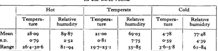
Three constant temperature rooms were used, maintained at temperatures of approximately 28, 21 and 50 C. Daily readings of temperature and relative humidity were taken in each room by means of a whirling hygrometer. Table 1 gives the

Table 1. Conditions of temperature (° C) and relative humidity in the three rooms

Mean S.D. Range

Hot

Tempera-ture

2809 079 26-4-30-6

Relative humidity

89-87 2-52 81-94

Temperate

Tempera-ture

21-00 o-8i 197-23.1

Relative humidity

69-03 7-75 55-85

Cold

Tempera-ture

4-78 059 3-6-5-8

Relative humidity

77-48 439 61-84

means, standard deviations and ranges of these readings for the period of the experiment. In addition, the temperature was continuously recorded in all three rooms, and in the cold room two maximum-minimum thermometers placed one

at either end of the room were read daily. Relative humidity was continuously recorded in the hot and temperate rooms throughout the experiment. In the hot and temperate rooms the air was circulated by a fan; in the temperate room the fan gave trouble, and had to be replaced by a faster moving fan at a stage in the experiment when the litters in the room were between 2 and 3 weeks of age. In the cold room the air was intermittently stirred by a fan. In the hot room the humidity was kept high and constant by placing trays of water in front of the fan.

Nulliparous female mice of Theiler's Original strain (TO strain), judged by external appearance to be pregnant, were obtained from the National Institute for Medical Research, Mill Hill, where they had been kept at a temperature of 20-21 ° C. The average stage of pregnancy was about 12^ days. By the use of a table of random numbers 30 females were allotted to the hot room, 29 to the cold room, and 20 to the temperate room. Those destined for the cold room were left overnight in a cool room (10-15-5° C). r^n e mice were kept singly in aluminium cages with open wire tops, and each received the same weighed amount of sawdust and cotton wool for bedding. The mice were fed ad lib on a standard pellet diet (M.R.C. diet no. 41).

The cages were examined each morning for births. The young mice were weighed individually on the day the litter was found and at weekly intervals for 4 weeks thereafter. Mice under 10 g. were weighed to o-oi of a g.; mice of 10 g. and over to o-i of a g. At the second weighing (1 week of age) the mice were sexed; at the third weighing (2 weeks of age) a note was made of whether or not the eyes were open, and at the final weighing (4 weeks of age) a note was made of whether or not the vaginas of the females were patent.

THE EXPERIMENTAL GENERATION

Twenty-four litters were born in the hot room, twenty in the cold room, and eighteen in the temperate room. The average litter sizes at birth (live + dead) were 7-04, 7-25 and 8-o6, respectively. The litter sizes in the hot and cold rooms proved to be more variable than those in the temperate room, significantly so in the case of the cold. This suggests that the small average litter sizes in the extreme environ-ments were a reflexion of increased prenatal mortality rather than an accident of sampling. This increase in prenatal mortality has been confirmed in a later experi-ment, and agrees with the work of Barnett & Manly (1956), who found that the average litter size of females from the C 57 BL inbred strain was strikingly reduced at — 30 C. as compared with 21 or io° C.

Certain litters and certain individual mice were omitted from the calculations on body weight for the following reasons.

(1) If a female stopped lactating, with the result that the litter actually decreased in mean weight in the course of a week, or if a water bottle flooded a cage, all weights of the litter subsequent to the cessation of lactation or to the flood were omitted.

(2) Because of the very humid atmosphere in the hot room, some of the newborn mice stuck to the cotton-wool bedding and were thereby injured. Such mice were killed.

(3) Occasionally mice were so stunted in growth that their weights fell outside the normal distribution of the rest of the litter. If such 'runts' or outliers are included in the statistical analysis, they can spuriously inflate the estimates of variability and invalidate tests of significance with respect to means. A test for outliers based upon the method of Dixon (1953) was therefore applied to all litters, and any outlying values were excluded from the calculations.

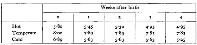
Table 2. Mean live titter size in the three environments

Hot Temperate Cold

Weeks after birth

0

5-8o 8-oo 6-89

1

5-45 7-89 5-63

2

5-3° 7-89 5-63

3

4-95 7-83 5-63

4

4-95 7-83 5-25

Table 2, which shows the mean live litter sizes for each week in each of the three rooms, illustrates the natural mortality occurring during the course of the experi-ment. For the purposes of this table runts have been included; litters which suffered flooding have been omitted altogether, and newborn mice damaged by sticking to the bedding in the hot room have been omitted, thus underestimating the mean litter size in the hot room throughout. Mortality was greater in the extreme environments than in the temperate, and greater in the cold room than in the hot In the cold room most of the deaths occurred during the first week of life; moreover, the deaths of three litters in toto during the first week can be added to the natural mortality indicated in Table 2. The number of litters and the number of mice of each sex actually available for analysis at each week is shown in Table 3.

Table 3. Numbers of titters and mice used in analysis of

body-weight data

Hot

Temperate

Cold

No. of litters No. of females No. of males No. of litters No. of females No. of males No. of litters No. of females No. of males

Weeks after birth

0

22 } 145

18

} 139

20

} • » •

1

22 56 61

18 65 68 16 44 45

2

19 46

5°

18 69 70 16 45 45

3

19 46 50 18 68 69 15 39 37

4

19 46 47 18 67 68

RESULTS AND THEIR ANALYSIS

Biometrical aspects

Scale. It is essential to decide at the outset on what scale we are to express body weight. One of the most important factors which affects this choice is that the various influences on the mean should act additively. There is evidence that in the case of growing mice the logarithmic scale satisfies this condition. Thus, Falconer (1953), in a long-term selection experiment for high and low 6-week weights, found that genetic differences act additively on the logarithmic scale.

The logarithmic transformation is indicated when there is a proportional relation-ship between the standard deviation and the mean when calculated on the arith-metic scale. This relation implies that the groups have constant coefficients of variation, and therefore equal standard deviations when expressed on the log-arithmic scale (Aitchison & Brown, 1957). If this is so, the usual analysis of variance procedures can be applied after transformation to the logarithmic scale. Evidence that this proportional relationship holds for the body weights of growing mice is provided by the results published by Chai (1956a, b). This worker measured 60-day weights of eight groups of mice of comparable genetic variability ranging from 14 to 37 g. in mean values, and found that the arithmetic standard deviations were proportional to the means. Also, Howard (personal communication), who took weekly weights from birth to 10 weeks of age in large samples of inbred and Fx hybrid mice, found proportionality between standard deviation and mean when comparing the different age groups for the first 4 weeks of life, the period to which our data relate. We have accordingly transformed all weights into logarithms for the calculation of means and other statistics. The test for outliers described earlier was carried out on the transformed data.

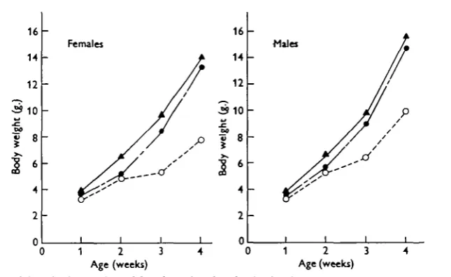
Crude growth curves. Fig. 1 shows the mean body weights in the three environ-ments week by week. The means were calculated on the logarithmic scale, but for graphic presentation have been reconverted into grammes. As explained in the next section, effects of environmental treatments cannot be accurately assessed from crude growth data uncorrected for litter size. On the other hand, the sex difference in growth, which is a constant feature of Fig. 1, is relatively unaffected by litter size. It attains significant proportions in all three environments and is in line with the generally observed fact that male mice grow faster than females (e.g. Falconer, 1953; Chai, 1956a). For this reason the two sexes are separately treated in the ensuing analysis.

Relation between body weight and litter size. The more mice there are in a Utter, the smaller they are at birth and the slower they grow. In comparing our growth data at different environmental temperatures we must take this effect into account, since early mortality substantially reduced the average litter sizes of the groups reared in the hot and cold environments as compared with those reared in the temperate environment. A weighted linear regression equation of the form:

is fitted to the data for each age group in each environment. yx is the expected mean log body weight for a Utter containing x mice; yw and xw denote weighted means, and the regression coefficient, b, states the amount by which the mean is on average changed by each additional mouse in the litter. In calculating the regression the weighting (10) given to each mean was the number of individuals contributing to it. The methods of calculation are described by Quenouille (1952).

To illustrate, we may take the data on 4-week mice raised in the cold (Table 4).

16

14

12

3 10

% 8

1

4

Femalei Males

1 1

Fig.

2 3 4 Age (weeks) Age (weeks)

Mean body weights of female and male mice in the three environments at 1—4 weeks of age. H o t , # • ; Temperate, A — A ; cold, O O.

Table 4. Specimen sheet of data required for calculating weighted regression

coefficients (4-week-old mice reared in the cold environment)

Litter no. 1 3 4 5 7 8* 1 0 1 2 1 3 1 4 1 5 1 9 2 0

2 3 * 27 Litter size (x) 7 3 7 3 1 0 7 7 5 2 4 4 3 6 4 8 No. («*) 4 2 3 3 3 1 2 2 2 3 3 3 2 3 2 Males Mean log weight Cv,;) 1-0593 1-1050 1-1883 1-2053 0-7847 [•0370 [•2085 [•2410 [•1655 •2560 •2043 • " 3 3 •1740 •3153 1-0370 Females No. (u>?) Mean log weight (y?)

3 1 I-OI47 I , 1-0790 4 i-"S7 0 — 7 5 5 0-7059 1-0178 1-1788 3 12237 0 _— I I2IOO I 0 4 0 6 1-1880 — 1-1595 — 1-0523

, runts were present in the litter and have been omitted. • When x > ^

Weighted regressions:

The fitted regression equations are shown at the foot of the table. Both coefficients are highly significant (001 >P>o-ooi), indicating a marked dependence of body weight on litter size. They are negative in sign, showing that the larger the number of individuals in the litter the smaller the mean body weight.

Since all weights have been transformed into logarithms, the regression coefficients are themselves logarithms. To interpret on the arithmetic scale we take anti-logarithms. Thus, in Table 4 the antilog of the regression coefficient for females is 0*83, and therefore in the cold each additional mouse present in a litter at 4 weeks decreases the expected mean weight in grammes of the females in the litter by 1-00 — 0-83, o r X7%- Similarly, in the males an additional mouse in a litter decreases the expected mean weight by about 9%.

4 5 6 Litter size

10

Fig. 2. Regression of mean log body weight upon litter size for 4-week-old female mice in the cold environment. The heights of the lines yt, yw and y, estimate the mean log body weight

cor-responding to litter size 6, the weighted mean litter size, and litter size 9, respectively.

In Fig. 2 the litter means for females have been plotted against litter sizes and the fitted regression line has been superimposed. There is a suggestion of curvi-linearity, and this is also found when the data on the males in Table 4 are similarly plotted. This may reflect the fact that in the cold some of the smallest litters at 4 weeks consisted of the survivors of initially large litters which had suffered catastrophic mortality. Such survivors might be expected to be stunted by the same factors which killed their sibs, and hence to fall below the fitted straight line at the left-hand end. Nevertheless, we have considered the use of linear regressions adequate for the limited purposes in view.

cannot be assumed independent.Thus simple tests of the homogeneity of parameters are not available. The following approximate method has therefore been adopted. Let m^ and wio be the mean log body weights of the males and females, respectively, in a Utter, and let there be 10^ males and w^ females. If there is no difference between the regressions associated with each sex we expect d=m^ — m^ to be constant for all litter sizes. This may be examined by calculating the weighted linear regression of d on litter size (x), the weighting attached to d being given by <w&. v>^\(y)$ + w?). This weighting factor gives greatest weight to those values of d calculated from litters with the largest numbers of mice, and from litters where the distribution of males and females tends to equality.

2-0 r

3

-10 Litter size

Fig. 3. Regression lines of mean log body weight upon litter size for 4-week-old females in the three environments, for the range of litter sizes encountered in each environment. Hot, • • ; temperate, • — A ; cold, O O.

The coefficient of the weighted regression of d on x, calculated from the data of Table 4, is 0-0063, D.F. 9, S.E. 00047, an£i ls n o t significantly different from zero. Hence, in this week and environment the relation between body weight and litter size does not differ significantly between the two sexes.

environ-nents is also shown. There axe considerable differences due to the differential mortality described earlier. It is seen that the range of litter sizes common to all environments is 6—9 inclusive, a rinding constant over all weeks. Thus, we have chosen to present mean log body weights for litter sizes at either end of the common range, i.e. litter sizes 6 and 9.

The biometrical methods illustrated above will now be applied to the assessment of the complete data.

Table 5. The mean log body weights for litter size 6 (j>6) and Utter size 9 (y9) and

the regression coefficients of mean log body weight on Utter-size (b), for each environment at each week

Sex Sexes combined Females Males Week o i 2 3 4 i 2 3 4 Environment Hot Temperate Cold Hot Temperate Cold Hot Temperate Cold Hot Temperate Cold Hot Temperate Cold Hot Temperate Cold Hot Temperate Cold Hot Temperate Cold Hot Temperate Cold y. O-2I 0-17 o-i4 0-62 o 63 0-62 0 8 5 o-88 o-86 I-O2 I-O4 0-97 1-19 1-17 1-13 0-62 o-6i 0-57 o-86 0 8 5 o-8i 1-04 i-oo 0-92 1-23 I-2I I - I I

y» 0-14 o-io O-II 0-56 o-6o 0-50

0 7 2 0 8 2

o-68 0-92 0-99 0-72 I - I 2 1-15 0-89

°-55 o-6o 0-52 0-76 0-82 0-72 0-95 0-99 o-8i 1-17

1 1 9

I'OO

b±th (DF.)

— 0-023 ±0-004 ( a o )# # #

— O-O24±O'OO2 (l6)**# — o o i 2 ± o - o o 3 (i8)#_**

— 0-019 ±0-007 (ao)#

— o-oi2±o-oio (15)

— 0-041 + 0-013 ( I I ) * *

— 0-043 ±o-oio (I_7)***

— o-020±o-oo8 (16)* — o-o59±o-oi5 ( 1 1 ) " — o-o32±o-oio (17)** - o o i 8 ± o - o o 8 ( i 6 )#

- 0 - 0 8 3 ±0-013 (9)*** — O-O2I ±O-OIO (17) — o-oo7±o-oo8 (16) - o - o 8 2 ± o - o i 8 ( 9 ) "

— o-o22± 0-007 (ao)*#

— 0-005 ±O-OI2 (16) — 0-015 ±o-oio (14) — o-O34±o-0ii ( 1 7 ) "

— O-OIO±O-OIO (16)

— o-030±o-oio (14)** — 0-027 ±o-o 10 (17)* — O-OO4±O-0I2 ( l 6 ) — o-o37±o-on (13)** — 0-020±0-0I0 (17) — o-oo5±o-on (16) — o-o39±o-oi2 (13)**

o-oi >P>o-ooi; P<o-ooi.

The complete data

The results can now be tabulated in a more illuminating form than the graphic presentation of crude growth curves. Table 5 gives means corrected to litter sizes 6 and 9 by the use of regression coefficients calculated separately for each group. The coefficients are also given, together with their standard errors and degrees of freedom.

upon litter size. Statistical tests of significance can be made between environments within each age group, since the data are independent, but these tests should not be used to compare ages within an environment since the data are serially correlated.

16

14

12

3 10

If 8

4

2

0

Females Males

1 2 3

Age (weeks) 1 2 3_{Age (weeks)}

Fig. 4. Mean body weights of female and male mice in the three environments at 1—4 weeks of age, corrected to litter size 6. Temperate, A — • ; hot, • • ; cold O O

Miles

,rt

1 2 3 Age (weeks)

1 2 3 Age (weeks)

Fig. 5. Mean body weights of female and male mice in the three environments at 1-4 weeks of age, corrected to litter size 9. Temperate, A—A; hot, • • ; cold, O O.

particularly for large litters, and the effect is significantly greater in females than in males. On the other hand, the difference between the mice reared in the hot and temperate environments is small and not significant.

Barnett & Manly (1956) found that the weight of mice 3 weeks of age was significantly depressed at — 30 C. in two out of three inbred strains tested, but not at io° C.

Comparison of regression coefficients. It seems reasonable to assume that the regression of log body weight on litter size is a measure of the degree of competition between individuals in a litter. Inspection of the values of b in Table 5 suggests that in the cold the effect of litter size is much more severe than in the other environments. The regression coefficients calculated from the weights at 4 weeks of both the male and female mice reared in the cold are significantly larger than the corresponding regression coefficients for the other environments. The development of this effect, week by week, is shown in Fig. 6. Although the graphs suggest strongly that the effect is more severe in the females there is no significant sex-difference in the regression coefficients at either week 3 or week 4 in any of the environments.

O

Males

O

4 0 1 2

Weeks

1 2 3

Weeks

Fig. 6. Regression coefficients of mean log body weight upon litter size, for female and male mice in the three environments at 1-4 weeks of age. Temperate, A—A; hot, • • ; cold O O.

In the case of the mice reared in the hot and temperate environments the litter-size effect reaches a peak at 2 weeks and then subsides. This might be expected since the peak corresponds to the period of greatest competition for the limited maternal food supply. But in the cold environment the effect is still increasing steeply at 4 weeks, suggesting that competition, and hence partial dependence on maternal lactation, is still continuing.

Effect on post-natal development

Table 6. The number of mice with open eyes at 2 weeks of age,

in each of the three climatic environments

Environment Hot Temperate Cold No. open 90 118 39 No. shut 0 3 45 Total 90 121 84

Table 7. The number of female mice with open vaginas at 4 weeks

of age, in each of the three environments

Environment Hot Temperate Cold Patent 17 16 3 Not patent 29 53 39 Total 46 69 42

different body-weight groups. The sexes were in agreement and have been com-bined. There is a clear tendency for the heavier mice to open their eyes earlier than the lighter ones. The females reared in the hot and temperate rooms are treated in the same way in Table 9 with respect to vaginal opening. Again rate of develop-ment is correlated with growth.

Table 8. Number of cold-reared mice with eyes open at 2 weeks of age,

arranged according to body weight

Eyes open Eyes shut

Total

Body weight (log grammes)

0-50-0-54 0 6 6 o-55-O59 0 5 5 o-6o-0-64 0 5 5 0^65-0-69 1 7 8 0-70-O-74 0 6 6 o-75-079 5 3 8 o-8o-0-84 4 4 8

0 8 5 -089 9 9 18 0-90-0-94 11 0 11 o-95-099 7 0 7 i-oo-1-04 2 0 2 Total 39 45 84

Table 9. Number of females reared in the hot and temperate rooms having

vaginas patent at 4 weeks of age, arranged according to body weight

Environ-ment Hot Temperate Vagina Patent Not patent Total Patent Not patent Total

Body weight (log grammes)

o-95-099 0 0 0 0 1 1 i-oo-1-04 0 1 1 0 1 1 1-05-1-09 1 5 6 0 10 10 I-IO-1 I-IO-1 4

2 4 6 0 15 15 1-15-119 0 9 6 17 33 I-2O-1-24 2 5 7 6 8 14

1 2 5 -1 2 9

SUMMARY

Pregnant mice were placed in rooms at three different environmental temperatures: hot, temperate and cold. The hot and cold environments were less favourable than the temperate as judged by incidence of both prenatal and postnatal mortality of the young. The growth and development of the young was studied during the first 4 weeks of life.

Body weight was expressed on the logarithmic scale throughout, and since males were found to be significantly heavier than females the two sexes were considered separately. The inverse relation between body weight and number of mice in a litter, reflecting competition between litter mates, was particularly marked in the cold and was still increasing 4 weeks after birth. In the hot and temperate environ-ments the effect reached a maximum at 2-3 weeks of age.

When allowance had been made for the effect of litter size on body weight, no significant differences in rate of growth or development were found between the mice in the hot and temperate environments. Both growth and development were markedly retarded in the cold.

We would like to express our thanks to Prof. N. J. Scorgie for the generous provision of facilities in his department, and in particular for the loan of the temperature-controlled rooms; to Prof. Scorgie, to Prof. E. C. Amoroso, F.R.S., and to Dr R. E. Glover, for the encouragement which they gave to this work; and to the Agricultural Research Council for financial support of two of us (A. M. and D. M.).

REFERENCES

AITCHMON, J. & BROWN, J. A. C. (1957). The Lognormal Distribution. Cambridge University Press. BARNETT, S. A. & MANLY, B. M. (1956). Reproduction and growth of mice of three strains, after

transfer to — 30 _{C. J. Exp. Biol. 33,}

325-^9-CHAI, C. K. (1956a). Analysis of quantitative inheritance of body size in mice. I. Hybridization and maternal influence. Genetics, 41, 157-64.

CHAI, C. K. (19566). Analysis of quantitative inheritance of body size in mice. II. Gene action and segregation. Genetics, 41, 165-78.

DIXON, W. J. (1953). Processing data for outliers. Biometrics, 9, 74-89.

FALCONER, D . S. (1953). Selection for large and small size in mice. J. Genet. 51, 470-501. MICHIE, D . (1955). Towards uniformity in experimental animals. Lab. Anim. Bur., collected

papers, 3,

37~47-MICHIE, D . , MCLAREN, A., ASHOUB, M. R. & BIGGERS, J. D . (1958) The effect of the environment on phenotypic variability. In preparation.