Haskell as a higher order structural hardware description language

Haskell as a higher order structural

hardware description language

Master's thesis

by

Matthijs Kooijman

December 9, 2009

Committee:

Dr. Ir. Jan Kuper

Ir. Marco Gerards

Ir. Bert Molenkamp

Dr. Ir. Sabih Gerez

Abstract

Functional hardware description languages have been around for a while, but never saw adoption on a large scale. Even though advanced features like higher order functions and polymorphism could enable very natural parametrization of hardware descriptions, the conventional hardware description languagesVHDL and Verilog are still most widely used.

Cλash is a new functional hardware description language using Haskell's syntax and semantics. It allows structurally describing synchronous hardware, using normal Haskell syntax combined with a selection of built-in functions for operations like addition or list operations. More complex constructions like higher order functions and polymorphism are fully supported.

Cλash supports stateful descriptions through explicit descriptions of a function's state. Every function accepts an argument containing its current state and returns its updated state as a part of its result. This means every function is called exactly once for each cycle, limiting Cλash to synchronous systems with a single clock domain.

A prototype compiler for Cλash has been implemented that can generate an equivalentVHDLdescription (using mostly structural VHDL). The prototype uses the front-end (parser, type-checker, desugarer) of the existingGHCHaskell compiler. This front-end generates aCoreversion of the description, which is a very small typed functional language. A normalizing system of transformations brings this Core version into a normal form that has any complex parts (higher order functions, polymorphism, complex nested structures) removed. The normal form can then be easily translated toVHDL. This design has proven to be very suitable. In particular the transformation system allows for some theoretical analysis and proofs about the compiler design itself (which have been left as future work).

Using Haskell syntax, semantics and existing tools has enabled the rapid creation of the prototype, but it also became clear that Haskell is not the ideal language for hardware specification. The problems encountered could be solved with syntax extensions and major improvements to Haskell's dependent typing support, or be circumvented entirely by developing a completely new language.

Acknowledgements

This thesis and the research it presents is not the result of just my own work. I have received a lot of ideas, inspiration and comments from other people, who I would like to mention here.

First of all, I would like to thank Christiaan Baaij, which has been my partner in crime during this research. Together we have started a new area of research at the University of Twente, in which I would not have progressed so far on my own.

Then there is my first supervisor, Jan Kuper, whose visions and ideas have sparked this research and who always managed to place my practical views into the proper theoretical background. The rest of the gradu-ation committee has been a great help, providing feedback, comments and challenging questions, each from their own unique point of view.

Contents

Introduction . . . 9

1 Context . . . 13

1.1 Conventional hardware description languages . . . 13

1.2 Existing functional hardware description languages . . . 13

2 Hardware description . . . 15

2.1 Function application . . . 15

2.2 Choice . . . 17

2.3 Types . . . 18

2.3.1 Built-in types . . . 19

2.3.2 User-defined types . . . 20

2.3.3 Partial application . . . 22

2.4 Costless specialization . . . 23

2.4.1 Specialization . . . 23

2.5 Higher order values . . . 24

2.6 Polymorphism . . . 24

2.7 State . . . 24

2.7.1 Approaches to state . . . 25

2.7.2 Explicit state specification . . . 27

2.7.3 Explicit state annotation . . . 28

2.8 Recursion . . . 28

2.8.1 List recursion . . . 29

2.8.2 General recursion . . . 30

3 Prototype . . . 31

3.1 Input language . . . 31

3.2 Output format . . . 31

3.3 Simulation and synthesis . . . 32

3.4 Prototype design . . . 32

3.5 The Core language . . . 34

3.5.1 Core type system . . . 39

3.6 State annotations in Haskell . . . 42

3.6.1 Type synonyms . . . 42

3.6.2 Type renaming (newtype) . . . 42

3.6.3 Type synonyms for sub-states . . . 43

3.6.4 Chosen approach . . . 44

3.7 VHDLgeneration for state . . . 44

3.7.1 State in normal form . . . 44

3.7.2 Translating toVHDL . . . 48

3.8 Prototype implementation . . . 50

4 Normalization . . . 53

4.1 Normal form . . . 53

4.1.1 Intended normal form definition . . . 56

4.2.1 Transformation application . . . 61

4.2.2 Definitions . . . 61

4.2.3 Binder uniqueness . . . 62

4.3 Transform passes . . . 63

4.3.1 General cleanup . . . 64

4.3.2 Program structure . . . 69

4.3.3 Representable arguments simplification . . . 73

4.3.4 Built-in functions . . . 75

4.3.5 Case normalization . . . 76

4.3.6 Removing unrepresentable values . . . 79

4.4 Unsolved problems . . . 87

4.4.1 Work duplication . . . 87

4.4.2 Non-determinism . . . 89

4.4.3 Casts . . . 89

4.4.4 Normalization of stateful descriptions . . . 89

4.5 Provable properties . . . 90

4.5.1 Graph representation . . . 91

4.5.2 Termination . . . 92

4.5.3 Soundness . . . 92

4.5.4 Completeness . . . 93

4.5.5 Determinism . . . 93

5 Future work . . . 95

5.1 New language . . . 95

5.2 Correctness proofs of the normalization system . . . 95

5.3 Improved notation for hierarchical state . . . 95

5.3.1 Breaking out of the Monad . . . 97

5.3.2 Alternative syntax . . . 98

5.3.3 Arrows . . . 98

5.4 Improved notation or abstraction for pipelining . . . 99

5.5 Recursion . . . 99

5.6 Multiple clock domains and asynchronicity . . . 100

5.7 Multiple cycle descriptions . . . 101

5.8 Higher order values in state . . . 103

5.9 Don't care values . . . 104

6 Conclusions . . . 107

Introduction

This thesis describes the result and process of my work during my Master's assignment. In these pages, I will introduce the world of hardware descriptions, the world of functional languages and compilers and introduce the hardware description language Cλash that will connect these worlds and puts a step towards making hardware programming on the whole easier, more maintainable and generally more pleasant. This assignment has been performed in close cooperation with Christiaan Baaij, whose Master's thesis [1] has been completed at the same time as this thesis. Where this thesis focuses on the interpretation of the Haskell language and the compilation process, [1] has a more thorough study of the field, explores more advanced types and provides a case study.

Research goals

This research started out with the notion that a functional program is very easy to interpret as a hardware description. A functional program typically makes no assumptions about evaluation order and does not have any side effects. This fits hardware nicely, since the evaluation order for hardware is simply everything in parallel.

As a motivating example, consider the simple functional program shown in example 11_{. This is a very natural} way to describe a lot of parallel not ports, that perform a bit-wise not on a bit-vector. The example also shows an image of the architecture described.

Example 1 Simple architecture that inverts a vector of bits.

notword :: [Bit] → [Bit] notword = map not

−−−→

input

not not not not

−−−−→

output

Haskell description of the architecture.

The architecture described by the Haskell description.

Slightly more complicated is the incremental summation of values shown in example 21_.

In this example we see a recursive functionsum'that recurses over a list and takes an accumulator argument that stores the sum so far. On each step of the recursion, another number from the input vector is added to the accumulator and each intermediate step returns its result.

This is a nice description of a series of sequential adders that produce the incremental sums of a vector of numbers. For an input list of length 4, the corresponding architecture is show in the example.

1

Introduction

Example 2 A recursive description that sums values.

sum :: [Int] → [Int] sum = sum' 0

sum' :: Int → [Int] → [Int] sum' acc [] = []

sum' acc (x:xs) = acc' : (sum' acc' xs) where acc' = x + acc

−−−→

input

0

+ + + + −−−−→output

Haskell description of the architecture. The architecture described by the Haskell description.

Or... is this the description of a single accumulating adder, that will add one element of each input each clock cycle and has a reset value of0? In that case, we would have described the architecture show in example 3

Example 3 An alternative interpretation of the description in example 2

input + output

The distinction in possible interpretations we see here, is an important distinction in this research. In the first figure, the recursion in the code is taken as recursion in space and each recursion step results in a different piece of hardware, all of which are active simultaneously. In the second figure, the recursion in the code is taken as recursion in time and each recursion step is executed sequentially,on the same piece of hardware. In this research we explore how to apply these two interpretations to hardware descriptions. Additionally, we explore how other functional programming concepts can be applied to hardware descriptions to give use an efficient way to describe hardware.

This leads us to the following research question:

“How can we describe the structural properties of a hardware design,

using a functional language?”

We can further split this into sub-questions from a hardware perspective:

Introduction

And sub-questions from a functional perspective:

• How to interpret recursion in descriptions?

• How to interpret polymorphism?

• How to interpret higher-order descriptions?

In addition to looking at designing a hardware description language, we will also implement a prototype to test ideas. This prototype will translate hardware descriptions written in the Haskell functional language to simple (netlist-like) hardware descriptions in theVHDLlanguage. The reasons for choosing these languages are detailed in section 3.1 and 3.2 respectively.

The name Cλash

The name Cλash more-or-less expands to CAES lan-guage for hardware descriptions, where CAES refers to the research chair where this project was under-taken (Computer Architectures for Embedded Sys-tems). The lambda in the name is of course a ref-erence to the lambda abstraction, which is an essen-tial element of most functional languages (and is also prominent in the Haskell logo).

Cλash is pronounced like ‘Clash'. The result of this research will thus be a prototype compiler and a

language that it can compile, to which we will refer to as the Cλash system and Cλash language for short, or simply Cλash.

Outline

In the first chapter, we will sketch the context for this research. The current state and history of hardware description languages will be briefly discussed, as well as the state and history of functional programming. Since we are not the first to have merged these ap-proaches, a number of other functional hardware description lan-guages are briefly described.

Chapter two describes the exploratory part of this research: how can we describe hardware using a functional language and how can we use functional concepts for hardware descriptions?

Chapter three talks about the prototype that was created and which has guided most of the research. There is some attention for the language chosen for our hardware descriptions, Haskell. The possibilities and limits of this prototype are further explored.

During the creation of the prototype, it became apparent that some structured way of doing program transfor-mations was required. Doing ad hoc interpretation of the hardware description proved non-scalable. These transformations and their application are the subject of the fourth chapter.

The next chapter sketches ideas for further research, which are many. Some of them have seen some initial exploration and could provide a basis for future work in this area.

1 Context

Embedded domain-specific languages (

)

An embeddedDSLis aDSLthat is embedded in another language. Haskell is commonly used to embedDSLs in, which typically means a number of Haskell functions and types are made available that can be called to con-struct a large value of some domain-specific datatype (e.g., a circuit datatype). This generated datatype can then be processed further by theEDSL‘compiler' (which runs in the same environment as theEDSLitself. The em-bedded language is then a, mostly applicative, subset of Haskell where the library functions are the primitives. Sometimes advanced Haskell features such as polymor-phism, higher-order values or type classes can be used in the embedded language. [3]

For anEDSL, the definitions of compile-time and run-time are typically fuzzy (and thus hard to define here), since the EDSL ‘compiler' is usually compiled by the same Haskell compiler as theEDSLprogram itself.

An obvious question that arises when starting any research is ‘Has this not been done before?'. Using a functional language for describing hardware is not a new idea at all. In fact, there has been research into functional hardware description even be-fore the conventional hardware description languages were cre-ated. Examples of these are µFP [4] and Ruby [5]. Functional languages were not nearly as advanced as they are now, and functional hardware description never really got off.

Recently, there have been some renewed efforts, especially us-ing the Haskell functional language. Examples are Lava [6] (an EDSL) and ForSyde [7] (anEDSLusing Template Haskell). [1] has a more complete overview of the current field.

We will now have a look at the existing hardware description languages, both conventional and functional to see the fields in which Cλash is operating.

1.1 Conventional hardware description languages

Considering that we already have some hardware description languages likeVHDLand Verilog, why would we need anything else? By introducing the functional style to hardware descrip-tion, we hope to obtain a hardware description language that is:

• More concise. Functional programs are known for their con-ciseness and ability to provide reusable functions that are

abstractions of common patterns. This is largely enabled by features like an advanced type system with polymorphism and higher-order functions.

• Type-safer. Functional programs typically have a highly expressive type system, which allows a pro-grammer to more strictly define limitations on values, making it easier to find violations and thus bugs.

purity p.25 • Easy to process. Functional languages have nice properties like purity and single binding behavior, which

make it easy to apply program transformations and optimizations and could potentially simplify program verification.

1.2 Existing functional hardware description languages

As noted above, this path has been explored before. However, current embedded functional hardware de-scription languages (in particular those using Haskell) are limited. Below a number of downsides are sketched of the recent attempts using the Haskell language. [1] has a more complete overview of these and other lan-guages.

1.2 — Context — Existing functional hardware description languages

Template Haskell

Template Haskell is an extension to the GHC compiler that allows a program to mark some parts to be evalu-ated at compile time. Thesetemplatescan then access the abstract syntax tree (AST) of the program that is be-ing compiled and generate parts of thisAST.

Template Haskell is a very powerful, but also complex mechanism. It was intended to simplify the generation of some repetitive pieces of code, but its introspection features have inspired all sorts of applications, such as hardware description compilers.

• Not all of Haskell's constructs can be captured by embed-ded domain specific languages. For example, aniforcase expression is typically executed once when the Haskell de-scription is processed and only the result is reflected in the generated data-structure (and thus in the final program). In Lava, for example, conditional assignment can only be de-scribed by using explicit multiplexer components, not using any of Haskell's compact mechanisms (such ascase expres-sions or pattern matching).

Also, sharing of variables (e.g., using the same variable twice while only calculating it once) and cycles in circuits are non-triv-ial to properly and safely translate (though there is some work to fix this, but that has not been possible in a com-pletely reliable way yet [8]).

• Template Haskell makes descriptions verbose. Template Haskell needs extra annotations to move things around betweenTHand the normal program. WhenTHis com-bined with anEDSLapproach, it can get confusing when to useTHand when not to.

• Function hierarchies cannot be observed in anEDSL. For example, Lava generates a single flatVHDL ar-chitecture, which has no structure whatsoever. Even though this is strictly correct, it offers no support to the synthesis software about which parts of the system can best be placed together and makes debugging the system very hard.

It is possible to add explicit annotation to overcome this limitation (ForSyDe does this using Template Haskell), but this adds extra verbosity again.

2 Hardware description

In this chapter an overview will be provided of the hardware description language that was created and the issues that have arisen in the process. The focus will be on the issues of the language, not the implementation. The prototype implementation will be discussed in chapter 3.

To translate Haskell to hardware, every Haskell construct needs a translation toVHDL. There are often multiple valid translations possible. When faced with choices, the most obvious choice has been chosen wherever possible. In a lot of cases, when a programmer looks at a functional hardware description it is completely clear what hardware is described. We want our translator to generate exactly that hardware whenever possible, to make working with Cλash as intuitive as possible.

Reading the examples

In this thesis, a lot of functional code will be presented. Part of this will be valid Cλash code, but others will just be small Haskell or Core snippets to illustrate a concept.

In these examples, some functions and types will be used, without properly defining every one of them. These func-tions (likeand,not,add,+, etc.) and types (likeBit,Word, Bool, etc.) are usually pretty self-explanatory.

The special type[t]means ‘list oft's', wheretcan be any other type.

Of particular note is the use of the:: operator. It is used in Haskell to explicitly declare the type of function or let binding. In these examples and the text, we will occasionally use this operator to show the type of arbitrary expressions, even where this would not normally be valid. Just reading the:: operator as ‘and also note thatthisexpression has thistype' should work out.

In this chapter we describe how to interpret a Haskell pro-gram from a hardware perspective. We provide a description of each Haskell language element that needs translation, to provide a clear picture of what is supported and how.

2.1 Function application

The basic syntactic elements of a functional program are functions and function application. These have a single ob-viousVHDLtranslation: each top level function becomes a hardware component, where each argument is an input port and the result value is the (single) output port. This output port can have a complex type (such as a tuple), so having just a single output port does not pose a limitation.

Each function application in turn becomes component in-stantiation. Here, the result of each argument expression is assigned to a signal, which is mapped to the corresponding input port. The output port of the function is also mapped to a signal, which is used as the result of the application.

Since every top level function generates its own component, the hierarchy of of function calls is reflected in the finalVHDLoutput as well, creating a hierarchicalVHDLdescription of the hardware. This separation in different components makes the resultingVHDLoutput easier to read and debug.

Example 2.1 shows a simple program using only function application and the corresponding architecture.

Example 2.1 Simple three input and gate.

-- A simple function that returns -- conjunction of three bits

and3 :: Bit -> Bit -> Bit -> Bit

and3 a b c = and (and a b) c a

b c

and

and out

2.1 — Hardware description — Function application

Example 2.2 VHDLgenerated forand3from example 2.1

entity and3Component_0 is

port (\azMyG2\ : in std_logic; \bzMyI2\ : in std_logic; \czMyK2\ : in std_logic;

\foozMySzMyS2\ : out std_logic; clock : in std_logic;

resetn : in std_logic); end entity and3Component_0;

architecture structural of and3Component_0 is signal \argzMyMzMyM2\ : std_logic; begin

\argzMyMzMyM2\ <= \azMyG2\ and \bzMyI2\;

2.2 — Hardware description — Choice

Top level binders and functions

Atop level binderis any binder (variable) that is de-clared in the ‘global' scope of a Haskell program (as opposed to a binder that is bound inside a function. The binder together with its body is referred to as a top level binding.

In Haskell, there is no sharp distinction between a variable and a function: a function is just a variable (binder) with a function type. This means that atop level functionis just any top level binder with a func-tion type. This also means that sometimes top level function will be used when top level binder is really meant.

As an example, consider the following Haskell snip-pet:

foo :: Int -> Int foo x = inc x

where

inc = \y -> y + 1

Here,foois a top level binder, whereasincis a func-tion (since it is bound to a lambda extracfunc-tion, indi-cated by the backslash) but is not a top level binder or function. Since the type offoois a function type, namelyInt -> Int, it is also a top level function.

2.2 Choice

Although describing components and connections allows us to de-scribe a lot of hardware designs already, there is an obvious thing missing: choice. We need some way to be able to choose between values based on another value. In Haskell, choice is achieved by caseexpressions,ifexpressions, pattern matching and guards. An obvious way to add choice to our language without having to recognize any of Haskell's syntax, would be to add a primitive ‘if' function. This function would take three arguments: the condition, the value to return when the condition is true and the value to return when the condition is false.

Thisiffunction would then essentially describe a multiplexer and allows us to describe any architecture that uses multiplexers. However, to be able to describe our hardware in a more convenient way, we also want to translate Haskell's choice mechanisms. The easiest of these are of course case expressions (andifexpressions, which can be very directly translated tocaseexpressions). Acase expression can in turn simply be translated to a conditional assign-ment, where the conditions use equality comparisons against the constructors in thecaseexpressions.

In example 2.3 two versions of an inverter are shown. The first uses a simplecaseexpression, scrutinizing a Boolean value. The corre-sponding architecture has a comparator to determine which of the constructors is on theininput. There is a multiplexer to select the output signal (which is just a conditional assignment in the gener-atedVHDL). The two options for the output signals are just constants, but these could have been more complex expressions (in which case also both of them would be working in parallel, regardless of which output would be chosen eventually). TheVHDLgenerated for (both versions of) this inverter is shown in example 2.4.

2.3 — Hardware description — Types

Arguments / results vs. inputs / outputs

Due to the translation chosen for function applica-tion, there is a very strong relation between argu-ments, results, inputs and outputs. For clarity, the former two will always refer to the arguments and results in the functional description (either Haskell or Core). The latter two will refer to input and out-put ports in the generatedVHDL.

Even though these concepts seem to be nearly iden-tical, when stateful functions are introduces we will see arguments and results that will not get translated into input and output ports, making this distinction more important.

A slightly more complex (but very powerful) form of choice is pat-tern matching. A function can be defined in multiple clauses, where each clause specifies a pattern. When the arguments match the pat-tern, the corresponding clause will be used.

Example 2.3 also shows an inverter that uses pattern matching. The architecture it describes is of course the same one as the description with a case expression. The general interpretation of pattern match-ing is also similar to that ofcaseexpressions: generate hardware for each of the clauses (like each of the clauses of acase expres-sion) and connect them to the function output through (a number of nested) multiplexers. These multiplexers are driven by compara-tors and other logic, that check each pattern in turn.

In these examples we have seen only binary case expressions and pattern matches (i.e., with two alternatives). In practice, case ex-pressions can choose between more than two values, resulting in a number of nested multiplexers.

Example 2.3 Simple inverter.

inv :: Bool -> Bool inv x = case x of

True -> False False -> True

Haskell description using a Case expression.

inv :: Bool -> Bool inv True = False inv False = True

Haskell description using Pattern matching expression.

in out True True False ==

The architecture described by the Haskell descriptions.

2.3 Types

Translation of two most basic functional concepts has been discussed: function application and choice. Before looking further into less obvious concepts like higher-order expressions and polymorphism, the possible types that can be used in hardware descriptions will be discussed.

Some way is needed to translate every values used to its hardware equivalents. In particular, this means a hardware equivalent for everytypeused in a hardware description is needed

2.3 — Hardware description — Types

Example 2.4 VHDLgenerated for (both versions of)invfrom example 2.3

entity invComponent_0 is

port (\xzAMo2\ : in boolean;

\reszAMuzAMu2\ : out boolean; clock : in std_logic;

resetn : in std_logic); end entity invComponent_0;

architecture structural of invComponent_0 is begin

\reszAMuzAMu2\ <= false when \xzAMo2\ = true else true;

end architecture structural;

hand, will have their hardware type derived directly from their Haskell declaration automatically, according to the rules sketched here.

2.3.1 Built-in types

The language currently supports the following built-in types. Of these, only theBooltype is supported by Haskell out of the box (the others are defined by the Cλash package, so they are user-defined types from Haskell's point of view).

Bit This is the most basic type available. It is mapped directly onto thestd_logicVHDLtype. Mapping this to thebittype might make more sense (since the Haskell version only has two values), but using std_logicis more standard (and allowed for some experimentation with don't care values)

Bool This is the only built-in Haskell type supported and is translated exactly like the Bit type (where a value ofTruecorresponds to a value ofHigh). Supporting the Bool type is particularly useful to support if ... then ... else ...expressions, which always have aBoolvalue for the condition. ABoolis translated to astd_logic, just likeBit.

SizedWord,SizedInt These are types to represent integers. ASizedWordis unsigned, while aSizedInt is signed. These types are parametrized by a length type, so you can define an unsigned word of 32 bits wide as follows:

type Word32 = SizedWord D32

Here, a type synonymWord32is defined that is equal to theSizedWordtype constructor applied to the typeD32.D32is thetype level representationof the decimal number 32, making theWord32type a 32-bit unsigned word.

2.3 — Hardware description — Types

Vector This is a vector type, that can contain elements of any other type and has a fixed length. It has two type parameters: its length and the type of the elements contained in it. By putting the length parameter in the type, the length of a vector can be determined at compile time, instead of only at run-time for conventional lists.

TheVectortype constructor takes two type arguments: the length of the vector and the type of the elements contained in it. The state type of an 8 element register bank would then for example be:

type RegisterState = Vector D8 Word32

Here, a type synonymRegisterStateis defined that is equal to theVectortype constructor applied to the typesD8(The type level representation of the decimal number 8) andWord32(The 32 bit word type as defined above). In other words, theRegisterStatetype is a vector of 8 32-bit words.

A fixed size vector is translated to aVHDLarray type.

RangedWord This is another type to describe integers, but unlike the previous two it has no specific bit-width, but an upper bound. This means that its range is not limited to powers of two, but can be any number. A RangedWordonly has an upper bound, its lower bound is implicitly zero. There is a lot of added imple-mentation complexity when adding a lower bound and having just an upper bound was enough for the primary purpose of this type: type-safely indexing vectors.

To define an index for the 8 element vector above, we would do:

type RegisterIndex = RangedWord D7

Here, a type synonym RegisterIndexis defined that is equal to theRangedWord type constructor applied to the typeD7. In other words, this defines an unsigned word with values from0 to 7(inclusive). This word can be be used to index the 8 element vectorRegisterStateabove.

This type is translated to theunsignedVHDLtype.

The integer and vector built-in types are discussed in more detail in [1].

2.3.2 User-defined types

There are three ways to define new types in Haskell: algebraic data-types with thedata keyword, type synonyms with thetypekeyword and type renamings with thenewtypekeyword. GHCoffers a few more advanced ways to introduce types (type families, existential typing, GADTs, etc.) which are not standard Haskell. These will be left outside the scope of this research.

2.3 — Hardware description — Types

Product types A product type is an algebraic datatype with a single constructor with two or more fields, denoted in practice like (a,b), (a,b,c), etc. This is essentially a way to pack a few values together in a record-like structure. In fact, the built-in tuple types are just algebraic product types (and are thus supported in exactly the same way).

The ‘product' in its name refers to the collection of values belonging to this type. The collection for a product type is the Cartesian product of the collections for the types of its fields.

These types are translated toVHDLrecord types, with one field for every field in the constructor. This translation applies to all single constructor algebraic data-types, including those with just one field (which are technically not a product, but generate a VHDL record for implementation simplicity).

Enumerated types An enumerated type is an algebraic datatype with multiple constructors, but none of them have fields. This is essentially a way to get an enumeration-like type containing alternatives. Note that Haskell'sBooltype is also defined as an enumeration type, but we have a fixed translation for that.

These types are translated toVHDLenumerations, with one value for each constructor. This allows refer-ences to these constructors to be translated to the corresponding enumeration value.

Sum types A sum type is an algebraic datatype with multiple constructors, where the constructors have one or more fields. Technically, a type with more than one field per constructor is a sum of products type, but for our purposes this distinction does not really make a difference, so this distinction is note made. The ‘sum' in its name refers again to the collection of values belonging to this type. The collection for a sum type is the union of the the collections for each of the constructors.

Sum types are currently not supported by the prototype, since there is no obviousVHDLalternative. They can easily be emulated, however, as we will see from an example:

data Sum = A Bit Word | B Word

An obvious way to translate this would be to create an enumeration to distinguish the constructors and then create a big record that contains all the fields of all the constructors. This is the same translation that would result from the following enumeration and product type (using a tuple for clarity):

data SumC = A | B

type Sum = (SumC, Bit, Word, Word)

Here, theSumCtype effectively signals which of the latter three fields of theSumtype are valid (the first two ifA, the last one ifB), all the other ones have no useful value.

An obvious problem with this naive approach is the space usage: the example above generates a fairly bigVHDLtype. Since we can be sure that the twoWords in theSumtype will never be valid at the same time, this is a waste of space.

2.3 — Hardware description — Types

Another interesting case is that of recursive types. In Haskell, an algebraic datatype can be recursive: any of its field types can be (or contain) the type being defined. The most well-known recursive type is probably the list type, which is defined is:

data List t = Empty | Cons t (List t)

Note thatEmptyis usually written as[]andConsas:, but this would make the definition harder to read. This immediately shows the problem with recursive types: what hardware type to allocate here?

If the naive approach for sum types described above would be used, a record would be created where the first field is an enumeration to distinguishEmptyfromCons. Furthermore, two more fields would be added: one with the (VHDLequivalent of) typet(assuming this type is actually known at compile time, this should not be a problem) and a second one with typeList t. The latter one is of course a problem: this is exactly the type that was to be translated in the first place.

The resulting VHDLtype will thus become infinitely deep. In other words, there is no way to statically determine how long (deep) the list will be (it could even be infinite).

In general, recursive types can never be properly translated: all recursive types have a potentially infinite value (even though in practice they will have a bounded value, there is no way for the compiler to automat-ically determine an upper bound on its size).

2.3.3 Partial application

Now the translation of application, choice and types has been discussed, a more complex concept can be considered: partial applications. Apartial applicationis any application whose (return) type is (again) a function type.

From this, it should be clear that the translation rules for full application does not apply to a partial application: there are not enough values for all the input ports in the resultingVHDL. Example 2.5 shows an example use of partial application and the corresponding architecture.

Example 2.5 Simple three port and.

-- Multiply the input word by four.

quadruple :: Word -> Word quadruple n = mul (mul n)

where

mul = (*) 2

n

2

× × out

Haskell description using function applications. The architecture described by the Haskell description.

2.4 — Hardware description — Costless specialization

However, it is clear that the above hardware description actually describes valid hardware. In general, any partial applied function must eventually become completely applied, at which point hardware for it can be generated using the rules for function application given in section 2.1. It might mean that a partial application is passed around quite a bit (even beyond function boundaries), but eventually, the partial application will become completely applied. An example of this principle is given in section 4.3.6.2.

2.4 Costless specialization

Each (complete) function application in our description generates a component instantiation, or a specific piece of hardware in the final design. It is interesting to note that each application of a function generates aseparatepiece of hardware. In the final design, none of the hardware is shared between applications, even when the applied function is the same (of course, if a particular value, such as the result of a function application, is used twice, it is not calculated twice).

This is distinctly different from normal program compilation: two separate calls to the same function share the same machine code. Having more machine code has implications for speed (due to less efficient caching) and memory usage. For normal compilation, it is therefore important to keep the amount of functions limited and maximize the code sharing (though there is a trade-off between speed and memory usage here). When generating hardware, this is hardly an issue. Having more ‘code sharing' does reduce the amount of VHDLoutput (Since different component instantiations still share the same component), but after synthesis, the amount of hardware generated is not affected. This means there is no trade-off between speed and memory (or rather, chip area) usage.

In particular, if we would duplicate all functions so that there is a separate function for every application in the program (e.g., each function is then only applied exactly once), there would be no increase in hardware size whatsoever.

Because of this, a common optimization technique calledspecializationcan be applied to hardware generation without any performance or area cost (unlike for software).

2.4.1 Specialization

Given some function that has adomainD(e.g., the set of all possible arguments that the function could be

applied to), we create a specialized function with exactly the same behavior, but with a domainD0 ⊂ D.

This subset can be chosen in all sorts of ways. Any subset is valid for the general definition of specialization, but in practice only some of them provide useful optimization opportunities.

Common subsets include limiting a polymorphic argument to a single type (i.e., removing polymorphism) or limiting an argument to just a single value (i.e., cross-function constant propagation, effectively removing the argument).

Since we limit the argument domain of the specialized function, its definition can often be optimized further (since now more types or even values of arguments are already known). By replacing any application of the function that falls within the reduced domain by an application of the specialized version, the code gets faster (but the code also gets bigger, since we now have two versions instead of one). If we apply this technique often enough, we can often replace all applications of a function by specialized versions, allowing the original function to be removed (in some cases, this can even give a net reduction of the code compared to the non-specialized version).

2.5 — Hardware description — Higher order values

specialized functions that remove the argument, or make it translatable, we can use specialization to make the original, untranslatable, function obsolete.

2.5 Higher order values

What holds for partial application, can be easily generalized to any higher-order expression. This includes partial applications, plain variables (e.g., a binder referring to a top level function), lambda expressions and more complex expressions with a function type (acaseexpression returning lambda's, for example). Each of these values cannot be directly represented in hardware (just like partial applications). Also, to make them representable, they need to be applied: function variables and partial applications will then eventually become complete applications, applied lambda expressions disappear by applying β-reduction, etc.

So any higher-order value will be ‘pushed down' towards its application just like partial applications. When-ever a function boundary needs to be crossed, the called function can be specialized.

2.6 Polymorphism

In Haskell, values can bepolymorphic: they can have multiple types. For example, the functionfst :: (a, b) -> ais an example of a polymorphic function: it works for tuples with any two element types. Haskell type classes allow a function to work on a specific set of types, but the general idea is the same. The opposite of this is amonomorphicvalue, which has a single, fixed, type.

When generating hardware, polymorphism cannot be easily translated. How many wires will you lay down for a value that could have any type? When type classes are involved, what hardware components will you lay down for a class method (whose behavior depends on the type of its arguments)? Note that Cλash currently does not allow user-defined type classes, but does partly support some of the built-in type classes (likeNum).

Fortunately, we can again use the principle of specialization: since every function application generates a separate piece of hardware, we can know the types of all arguments exactly. Provided that existential typing (which is aGHCextension) is not used typing, all of the polymorphic types in a function must depend on the types of the arguments (In other words, the only way to introduce a type variable is in a lambda abstraction). If a function is monomorphic, all values inside it are monomorphic as well, so any function that is applied within the function can only be applied to monomorphic values. The applied functions can then be specialized to work just for these specific types, removing the polymorphism from the applied functions as well.

The entry function must not have a polymorphic type (otherwise no hardware interface could be generated for the entry function).

By induction, this means that all functions that are (indirectly) called by our top level function (meaning all functions that are translated in the final hardware) become monomorphic.

2.7 State

2.7 — Hardware description — State

To make Cλash useful to describe more than simple combinational designs, it needs to be able to describe state in some way.

2.7.1 Approaches to state

In Haskell, functions are always pure (except when using unsafe functions with theIOmonad, which is not supported by Cλash). This means that the output of a function solely depends on its inputs. If you evaluate a given function with given inputs, it will always provide the same output.

Purity

A function is said to be pure if it satisfies two condi-tions:

I. When a pure function is called with the same ar-guments twice, it should return the same value in both cases.

II. When a pure function is called, it should have not observable side-effects.

Purity is an important property in functional lan-guages, since it enables all kinds of mathematical rea-soning and optimizations with pure functions, that are not guaranteed to be correct for impure func-tions.

An example of a pure function is the square root functionsqrt. An example of an impure function is thetodayfunction that returns the current date (which of course cannot exist like this in Haskell). This is a perfect match for a combinational circuit, where the output

also solely depends on the inputs. However, when state is involved, this no longer holds. Of course this purity constraint cannot just be removed from Haskell. But even when designing a completely new (hardware description) language, it does not seem to be a good idea to remove this purity. This would that all kinds of interesting properties of the functional language get lost, and all kinds of trans-formations and optimizations are no longer be meaning preserving. So our functions must remain pure, meaning the current state has to be present in the function's arguments in some way. There seem to be two obvious ways to do this: adding the current state as an argument, or including the full history of each argument.

2.7.1.1 Stream arguments and results

Including the entire history of each input (e.g., the value of that in-put for each previous clock cycle) is an obvious way to make outin-puts depend on all previous input. This is easily done by making every input a list instead of a single value, containing all previous values as well as the current value.

An obvious downside of this solution is that on each cycle, all the

previous cycles must be resimulated to obtain the current state. To do this, it might be needed to have a recursive helper function as well, which might be hard to be properly analyzed by the compiler.

A slight variation on this approach is one taken by some of the other functionalHDLs in the field: Make functions operate on complete streams. This means that a function is no longer called on every cycle, but just once. It takes stream as inputs instead of values, where each stream contains all the values for every clock cycle since system start. This is easily modeled using an (infinite) list, with one element for each clock cycle. Since the function is only evaluated once, its output must also be a stream. Note that, since we are working with infinite lists and still want to be able to simulate the system cycle-by-cycle, this relies heavily on the lazy semantics of Haskell.

Since our inputs and outputs are streams, all other (intermediate) values must be streams. All of our primitive operators (e.g., addition, subtraction, bit-wise operations, etc.) must operate on streams as well (note that changing a single-element operation to a stream operation can done withmap,zipwith, etc.).

This also means that primitive operations from an existing language such as Haskell cannot be used directly (including some syntax constructs, likecaseexpressions andifexpressions). This makes this approach well

EDSL p.13 suited for use inEDSLs, since those already impose these same limitations.

2.7 — Hardware description — State

can "look into" the past. Thisdelayfunction simply outputs a stream where each value is the same as the input value, but shifted one cycle. This causes a ‘gap' at the beginning of the stream: what is the value of the delay output in the first cycle? For this, thedelayfunction has a second input, of which only a single value is used.

Example 2.6 shows a simple accumulator expressed in this style.

Example 2.6 Simple accumulator architecture.

acc :: Stream Word -> Stream Word acc in = out

where

out = (delay out 0) + in in + out

Haskell description using streams. The architecture described by the Haskell description.

This notation can be confusing (especially due to the loop in the definition of out), but is essentially easy to interpret. There is a single call to delay, resulting in a circuit with a single register, whose input is connected toout(which is the output of the adder), and its output is the expressiondelay out 0(which is connected to one of the adder inputs).

2.7.1.2 Explicit state arguments and results

A more explicit way to model state, is to simply add an extra argument containing the current state value. This allows an output to depend on both the inputs as well as the current state while keeping the function pure (letting the result depend only on the arguments), since the current state is now an argument.

In Haskell, this would look like example 2.71_.

Example 2.7 Simple accumulator architecture.

-- input -> current state -> (new state, output)

acc :: Word -> Word -> (Word, Word) acc in s = (s', out)

where

out = s + in

s' = out in + out

2.7 — Hardware description — State

This approach makes a function's state very explicit, which state variables are used by a function can be completely determined from its type signature (as opposed to the stream approach, where a function looks the same from the outside, regardless of what state variables it uses or whether it is stateful at all).

This approach to state has been one of the initial drives behind this research. Unlike a stream based approach it is well suited to completely use existing code and language features (likeifandcaseexpressions) because it operates on normal values. Because of these reasons, this is the approach chosen for Cλash. It will be examined more closely below.

2.7.2 Explicit state specification

The concept of explicit state has been introduced with some examples above, but what are the implications of this approach?

2.7.2.1 Substates

Since a function's state is reflected directly in its type signature, if a function calls other stateful functions (e.g., has sub-circuits), it has to somehow know the current state for these called functions. The only way to do this, is to put thesesubstatesinside the caller's state. This means that a function's state is the sum of the states of all functions it calls, and its own state. This sum can be obtained using something simple like a tuple, or possibly custom algebraic types for clarity.

This also means that the type of a function (at least the "state" part) is dependent on its own implementation and of the functions it calls.

This is the major downside of this approach: the separation between interface and implementation is limited. However, since Cλash is not very suitable for separate compilation this is not a big problem in practice. Additionally, when using a type synonym for the state type of each function, we can still provide explicit type signatures while keeping the state specification for a function near its definition only.

2.7.2.2 Which arguments and results are stateful?

We need some way to know which arguments should become input ports and which argument(s?) should become the current state (e.g., be bound to the register outputs). This does not hold just for the top level function, but also for any sub-function. Or could we perhaps deduce the statefulness of sub-functions by analyzing the flow of data in the calling functions?

To explore this matter, the following observation is interesting: we get completely correct behavior when we put all state registers in the top level entity (or even outside of it). All of the state arguments and results on sub-functions are treated as normal input and output ports. Effectively, a stateful function results in a stateless hardware component that has one of its input ports connected to the output of a register and one of its output ports connected to the input of the same register.

Of course, even though the hardware described like this has the correct behavior, unless the layout tool does smart optimizations, there will be a lot of extra wire in the design (since registers will not be close to the component that uses them). Also, when working with the generatedVHDLcode, there will be a lot of extra ports just to pass on state values, which can get quite confusing.

2.8 — Hardware description — Recursion

inside the sub-circuit instead. This is slightly less trivial when looking at the Haskell code instead of the resulting circuit, but the idea is still the same.

However, when applying this technique, we might push registers down too far. When you intend to store a result of a stateless sub-function in the caller's state and pass the current value of that state variable to that same function, the register might get pushed down too far. It is impossible to distinguish this case from similar code where the called function is in fact stateful. From this we can conclude that we have to either:

• accept that the generated hardware might not be exactly what we intended, in some specific cases. In most cases, the hardware will be what we intended.

• explicitly annotate state arguments and results in the input description.

The first option causes (non-obvious) exceptions in the language interpretation. Also, automatically deter-mining where registers should end up is easier to implement correctly with explicit annotations, so for these reasons we will look at how this annotations could work.

2.7.3 Explicit state annotation

To make our stateful descriptions unambiguous and easier to translate, we need some way for the developer to describe which arguments and results are intended to become stateful.

Roughly, we have two ways to achieve this:

I. Use some kind of annotation method or syntactic construction in the language to indicate exactly which argument and (part of the) result is stateful. This means that the annotation lives ‘outside' of the function, it is completely invisible when looking at the function body.

II. Use some kind of annotation on the type level,i.e.give stateful arguments and stateful (parts of) results a different type. This has the potential to make this annotation visible inside the function as well, such that when looking at a value inside the function body you can tell if it is stateful by looking at its type. This could possibly make the translation process a lot easier, since less analysis of the program flow might be required.

From these approaches, the type level ‘annotations' have been implemented in Cλash. Section 3.6 expands on the possible ways this could have been implemented.

2.8 Recursion

An important concept in functional languages is recursion. In its most basic form, recursion is a definition that is described in terms of itself. A recursive function is thus a function that uses itself in its body. This usually requires multiple evaluations of this function, with changing arguments, until eventually an evaluation of the function no longer requires itself.

2.8 — Hardware description — Recursion

This is expected for functions that describe infinite recursion. In that case, we cannot generate hardware that shows correct behavior in a single cycle (at best, we could generate hardware that needs an infinite number of cycles to complete).

null

,

head

and

tail

The functions null, head and tail are common list functions in Haskell. Thenullfunction simply checks if a list is empty. Theheadfunction returns the first element of a list. Thetailfunction returns containing everythingexcept the first element of a list.

In Cλash, there are vector versions of these functions, which do exactly the same.

However, most recursive definitions will describe finite recursion. This is because the recursive call is done conditionally. There is usually acaseexpression where at least one alternative does not contain the recursive call, which we call the "base case". If, for each call to the recursive function, we would be able to detect at com-pile time which alternative applies, we would be able to remove the caseexpression and leave only the base case when it applies. This will ensure that expanding the recursive functions will terminate after a bounded number of expansions.

This does imply the extra requirement that the base case is de-tectable at compile time. In particular, this means that the decision between the base case and the recursive case must not depend on run-time data.

2.8.1 List recursion

The most common deciding factor in recursion is the length of a list that is passed in as an argument. Since we represent lists as vectors that encode the length in the vector type, it seems easy to determine the base case. We can simply look at the argument type for this. However, it turns out that this is rather non-trivial to write down in Haskell already, not even looking at translation. As an example, we would like to write down something like this:

sum :: Vector n Word -> Word sum xs = case null xs of

True -> 0

False -> head xs + sum (tail xs)

However, the Haskell type-checker will now use the following reasoning. For simplicity, the element type of a vector is left out, all vectors are assumed to have the same element type. Below, we write conditions on type variables before the=>operator. This is not completely valid Haskell syntax, but serves to illustrate the type-checker reasoning. Also note that a vector can never have a negative length, soVector nimplicitly means(n >= 0) => Vector n.

• tail has the type(n > 0) => Vector n -> Vector (n - 1)

• This means that xs must have the type(n > 0) => Vector n

• This means that sum must have the type(n > 0) => Vector n -> a(The typeais can be anything at this stage, we will not try to finds its actual type in this example).

2.8 — Hardware description — Recursion

• This means that sum must have the typeVector n -> a

• This is a contradiction between the type deduced from the body of sum (the input vector must be non-empty) and the use of sum (the input vector could have any length).

As you can see, using a simplecaseexpression at value level causes the type checker to always type-check both alternatives, which cannot be done. The type-checker is unable to distinguish the two case alternatives (this is partly possible usingGADTs, but that approach faced other problems [1]).

This is a fundamental problem, that would seem perfectly suited for a type class. Considering that we need to switch between to implementations of the sum function, based on the type of the argument, this sounds like the perfect problem to solve with a type class. However, this approach has its own problems (not the least of them that you need to define a new type class for every recursive function you want to define).

2.8.2 General recursion

Of course there are other forms of recursion, that do not depend on the length (and thus type) of a list. For example, simple recursion using a counter could be expressed, but only translated to hardware for a fixed number of iterations. Also, this would require extensive support for compile time simplification (constant propagation) and compile time evaluation (evaluation of constant comparisons), to ensure non-termination. Supporting general recursion will probably require strict conditions on the input descriptions. Even then, it will be hard (if not impossible) to really guarantee termination, since the user (orGHCdesugarer) might use some obscure notation that results in a corner case of the simplifier that is not caught and thus non-termina-tion.

3 Prototype

An important step in this research is the creation of a prototype compiler. Having this prototype allows us to apply the ideas from the previous chapter to actual hardware descriptions and evaluate their usefulness. Having a prototype also helps to find new techniques and test possible interpretations.

Obviously the prototype was not created after all research ideas were formed, but its implementation has been interleaved with the research itself. Also, the prototype described here is the final version, it has gone through a number of design iterations which we will not completely describe here.

3.1 Input language

When implementing this prototype, the first question to ask is: Which (functional) language will be used to describe our hardware? (Note that this does not concern theimplementation languageof the compiler, just the languagetranslated bythe compiler).

Initially, we have two choices:

• Create a new functional language from scratch. This has the advantage of having a language that contains exactly those elements that are convenient for describing hardware and can contain special constructs that allows our hardware descriptions to be more powerful or concise.

• Use an existing language and create a new back-end for it. This has the advantage that existing tools can be reused, which will speed up development.

No

or Template Haskell

Note that in this consideration, embedded domain-spe-cific languages (EDSL) and Template Haskell (TH) ap-proaches have not been included. As we have seen in section 1.2, these approaches have all kinds of lim-itations on the description language that we would like to avoid.

Considering that we required a prototype which should be work-ing quickly, and that implementwork-ing parsers, semantic checkers and especially type-checkers is not exactly the core of this research (but it is lots and lots of work, using an existing language is the obvi-ous choice. This also has the advantage that a large set of language features is available to experiment with and it is easy to find which features apply well and which do not. Another important advan-tage of using an existing language, is that simulation of the code becomes trivial. Since there are existing compilers and interpreters that can run the hardware description directly, it can be simulated without also having to write an interpreter for the new language.

A possible second prototype could use a custom language with just the useful features (and possibly extra features that are specific to the domain of hardware description as well).

The second choice to be made is which of the many existing languages to use. As mentioned before, the chosen language is Haskell. This choice has not been the result of a thorough comparison of languages, for the simple reason that the requirements on the language were completely unclear at the start of this research. The fact that Haskell is a language with a broad spectrum of features, that it is commonly used in research projects and that the primary compiler, GHC, provides a high level API to its internals, made Haskell an obvious choice.

3.2 Output format

3.3 — Prototype — Simulation and synthesis

Looking at other tools in the industry, the Electronic Design Interchange Format (EDIF) is commonly used for storing intermediatenetlists(lists of components and connections between these components) and is commonly the target forVHDLand Verilog compilers.

However,EDIFis not completely tool-independent. It specifies a meta-format, but the hardware components that can be used vary between various tool and hardware vendors, as well as the interpretation of theEDIF standard. [9]

This means that when working withEDIF, our prototype would become technology dependent (e.g. only work withFPGAs of a specific vendor, or even only with specific chips). This limits the applicability of our prototype. Also, the tools we would like to use for verifying, simulating and draw pretty pictures of our output (like Precision, or QuestaSim) are designed forVHDLor Verilog input.

For these reasons, we will not useEDIF, butVHDLas our output language. We choose VHDLover Verilog simply because we are familiar withVHDLalready. The differences betweenVHDLand Verilog are on the higher level, while we will be usingVHDLmainly to write low level, netlist-like descriptions anyway. An added advantage of usingVHDLis that we can profit from existing optimizations inVHDLsynthesizers. A lot of optimizations are done on theVHDLlevel by existing tools. These tools have been under development for years, so it would not be reasonable to assume we could achieve a similar amount of optimization in our prototype (nor should it be a goal, considering this is just a prototype).

Translation vs. compilation vs. synthesis

In this thesis the wordstranslation,compilationand sometimessynthesiswill be used interchangeably to refer to the process of translating the hardware de-scription from the Haskell language to theVHDL lan-guage.

Similarly, the prototype created is referred to as both thetranslatoras well as thecompiler.

The final part of this process is usually referred to as VHDLgeneration.

Note that we will be usingVHDLas our output language, but will not use its full expressive power. Our output will be limited to us-ing simple, structural descriptions, without any complex behavioral descriptions like arbitrary sequential statements (which might not be supported by all tools). This ensures that any tool that works withVHDLwill understand our output. This also leaves open the option to switch toEDIFin the future, with minimal changes to the prototype.

3.3 Simulation and synthesis

As mentioned above, by using the Haskell language, we get simu-lation of our hardware descriptions almost for free. The only thing that is needed is to provide a Haskell implementation of all built-in functions that can be used by the Haskell interpreter to simulate them.

The main topic of this thesis is therefore the path from the Haskell hardware descriptions toFPGAsynthesis, focusing of course on theVHDLgeneration. Since theVHDLgeneration process preserves the meaning of the Haskell description exactly, any simulation done in Haskellshouldproduce identical results as the synthesized hardware.

3.4 Prototype design

3.4 — Prototype — Prototype design

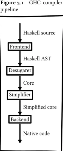
Figure 3.1 GHC compiler pipeline

Haskell source

Frontend

Haskell AST

Desugarer

Core

Simplifier

Simplified core

Backend

Native code

Frontend This step takes the Haskell source files and parses them into an abstract syntax tree (AST). ThisASTcan express the complete Haskell lan-guage and is thus a very complex one (in contrast with the CoreAST, later on). All identifiers in thisASTare resolved by the renamer and all types are checked by the type-checker.

Desugaring This step takes the fullASTand translates it to theCorelanguage. Core is a very small functional language with lazy semantics, that can still express everything Haskell can express. Its simpleness makes Core very suitable for further simplification and translation. Core is the language we will be working with as well.

Simplification Through a number of simplification steps (such as inlining, common sub-expression elimination, etc.) the Core program is simplified to make it faster or easier to process further.

Backend This step takes the simplified Core program and generates an actual runnable program for it. This is a big and complicated step we will not discuss it any further, since it is not relevant to our prototype.

In this process, there are a number of places where we can start our work. As-suming that we do not want to deal with (or modify) parsing, type-checking and other front end business and that native code is not really a useful for-mat anymore, we are left with the choice between the full HaskellAST, or the smaller (simplified) Core representation.

The advantage of taking the fullASTis that the exact structure of the source

program is preserved. We can see exactly what the hardware description looks like and which syntax con-structs were used. However, the fullASTis a very complicated data-structure. If we are to handle everything it offers, we will quickly get a big compiler.

Using the Core representation gives us a much more compact data-structure (a Core expression only uses 9 constructors). Note that this does not mean that the Core representation itself is smaller, on the contrary. Since the Core language has less constructs, most Core expressions are larger than the equivalent versions in Haskell.

However, the fact that the Core language is so much smaller, means it is a lot easier to analyze and translate it into something else. For the same reason, GHCruns its simplifications and optimizations on the Core representation as well [10].

3.5 — Prototype — The Core language

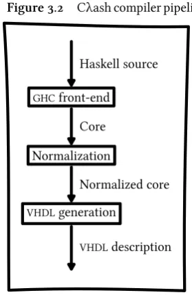
Figure 3.2 Cλash compiler pipeline

Haskell source

GHCfront-end

Core

Normalization

Normalized core

VHDLgeneration

VHDLdescription The final prototype roughly consists of three steps:

Frontend This is exactly the front-end from theGHCpipeline, that trans-lates Haskell sources to a typed Core representation.

Normalization This is a step that transforms the Core representation into a normal form. This normal form is still expressed in the Core language, but has to adhere to an additional set of constraints. This normal form is less expressive than the full Core language (e.g., it can have limited higher-order expressions, has a specific structure, etc.), but is also very close to directly describing hardware.

VHDLgeneration The last step takes the normal formed Core represen-tation and generatesVHDLfor it. Since the normal form has a specific, hardware-like structure, this final step is very straightforward.

The most interesting step in this process is the normalization step. That is where more complicated functional constructs, which have no direct hardware interpretation, are removed and translated into hardware con-structs. This step is described in a lot of detail at chapter 4.

Translation of a hardware description always starts at a single function, which is referred to as theentry function. VHDLis generated for this function first, followed by any functions used by the entry functions (recursively).

3.5 The Core language

Most of the prototype deals with handling the program in the Core language. In this section we will show what this language looks like and how it works.

The Core language is a functional language that describesexpressions. Every identifier used in Core is called abinder, since it is bound to a value somewhere. On the highest level, a Core program is a collection of functions, each of which bind a binder (the function name) to an expression (the function value, which has a function type).

The Core language itself does not prescribe any program structure (like modules, declarations, imports, etc.), only expression structure. In theGHCcompiler, the Haskell module structure is used for the resulting Core code as well. Since this is not so relevant for understanding the Core language or the Normalization process, we will only look at the Core expression language here.

Each Core expression consists of one of these possible expressions.

Variable reference

3.5 — Prototype — The Core language

scope, so a reference to a top level function is also a variable reference). Additionally, constructors from algebraic data-types also become variable references (e.g.True).

In our examples, binders will commonly consist of a single characters, but they can have any length. The value of this expression is the value bound to the given binder.

Each binder also carries around its type (explicitly shown above), but this is usually not shown in the Core expressions. Only when the type is relevant (when a new binder is introduced, for example) will it be shown. In other cases, the type is either not relevant, or easily derived from the context of the expression.

Literal

10

This is a literal. Only primitive types are supported, like chars, strings, integers and doubles. The types of these literals are the ‘primitive', unboxed versions, likeChar#andWord#, not the normal Haskell versions (but there are built-in conversion functions). Without going into detail about these types, note that a few conversion functions exist to convert these to the normal (boxed) Haskell equivalents. See section 4.3.6.3 for an example.

Application

func arg

This is function application. Each application consists of two parts: the function part and the argument part. Applications are used for normal function ‘calls', but also for applying type abstractions and data constructors.

The value of an application is the value of the function part, with the first argument binder bound to the argument part.

In Core, there is no distinction between an op