A Technique for Pulse RADAR Detection Using RRBF Neural Network

A Technique for Pulse RADAR Detection Using

RRBF Neural Network

Ajit Kumar Sahoo, Ganapati Panda and Babita Majhi

Abstract—Pulse compression technique combines the high

energy characteristic of a longer pulse width with the high resolution characteristic of a narrower pulse width. The major aspects that are considered for a pulse compression technique are signal to sidelobe ratio (SSR), noise and Doppler shift performances. The traditional algorithms like autocorrelation function (ACF), recursive least square (RLS) algorithm, multilayer perceptron (MLP), radial basis function (RBF) and recurrent neural network (RNN) have been applied for pulse compression and their performances have also been studied. This paper presents a new approach for pulse compression using recurrent radial Basis function (RRBF) neural network. 13 and 35-bit Barker codes are taken as input to RRBF network for pulse compression and the results are compared with MLP, RNN and RBF network based pulse compression schemes. The analysis of simulation results reveals that RRBF yields higher SSR, improved noise performance, better Doppler tolerance and hence more robust for pulse radar detection compared to the other techniques.

Index Terms—Pulse compression, SSR, Doppler shift, RRBF,

Barker code.

I. INTRODUCTION

Pulse compression plays a significant role in radar systems in achieving good signal strength and high range resolution. The good signal strength is achieved by long duration pulses, which reduces the peak power. Transmitting longer pulse increases the sensitivity of radar system by increasing the average transmitted power. But the longer pulse deteriorates the range resolution of the radar. For limited target classification, range resolution should be high enough which is obtained by narrow pulses. Hence as a compromise, pulse compression technique is employed in which a long duration pulse is either frequency or phase modulated to increase the bandwidth. This long duration modulated pulse is compressed at the receiver end using matched filter [1]. The SSR, noise and Doppler tolerance performances must be considered as major performance indices for a pulse compression technique. Based on these considerations many pulse compression techniques have been evolved.

Zrnik et. al [2] proposed a self-clutter suppression filter design using the modified recursive least square (RLS) algorithm which exhibits better performance as compared to iterative RLS and ACF algorithms. To suppress the sidelobes of Barker code of length 13, an adaptive finite impulse

Manuscript received March 06, 2012; revised March 29, 2012. Ajit Kumar Sahoo is with the Department of Electronics and Communication Engineering, National Institute of Technology, Rourkela, Orissa, India e-mail:ajitsahoo1@gmail.com

Ganapati Panda is with the School of Electrical Sciences, Indian Institute of Technology, Bhubaneswar, Orissa, India e-mail:ganapati.panda@gmail.com

Babita Majhi is with the Department of Computer Science and Information Technology G. G. Vishwavidyalaya(Central University), Bilaspur,Chhattisgarh, India e-mail:babita.majhi@gmail.com

response (FIR) filter is placed next to a matched filter pulse [3] and the filter is implemented via two approaches: Least Mean Square (LMS) and RLS algorithms. Kwan and Lee [4] used an MLP network for pulse radar detection to suppress the unwanted clutter. A RNN approach which yielded better SSR than MLP and autocorrelation approach is reported in [5]. Khairnar et. al [6] developed a RBF network which converges faster with higher SSRs in adverse situations of noise and better robustness in Doppler shift tolerance than MLP and other traditional algorithms like ACF algorithm. In recent literature there are other better performing algorithms which can be replacement for these traditionally used algorithms for pulse compression. It becomes interesting to examine the scope of further improvement in performance in terms of SSR, error convergence speed and Doppler shift in pulse compression system. In this paper, a new approach for radar pulse compression which uses RRBF is proposed. The simulation studies of the proposed technique are carried out to obtain various performance indices and the results of simulation are then compared with those obtained by RBF, RNN, MLP and ACF based pulse compression systems.

This paper is organized as follows. Section II discusses on the RBF and RRBF network and their learning algorithm. In Section III the performance of RRBF network is compared with those obtained by ACF, MLP, RNN and RBF. The concluding remarks are provided in Section IV.

II. RBFANDRRBF

A. Radial basis function

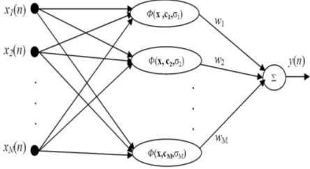
The radial basis function network can be viewed as a feed forward neural network with a single hidden layer which computes the distance between input pattern and the center [7]. It consists of three layers, an input layer, a hidden layer and an output layer. The input layer connects the network to the environment. The second layer is the only hidden layer which transfer the input space nonlinearly using radial basis function. The hidden space is greater than the input space in most of the applications. The response of the network provided by the output layer which is linear in nature. The RBF network is suitable for solving function approximation, system identification and pattern classification because of its simple topological structure and their ability to learn in an explicit manner [8], [9].

Fig. 1. Architecture of radial basis function network

Learning algorithm for RBF network

The error for thenth _{pattern is obtained as}

e(n) =d(n)− M

X

k=1

wk(m)φ(x(n),c_k(m), σ_k(m))) (1)

where d(n) is the desired output. If the Gaussian function chosen as the radial basis function

e(n) =d(n)− M

X

k=1

wk(m)exp −

kx(n)−c_k(m)k2 σ2

k(m)

!

(2)

The cost function is defined as

ξ= 1 2

n₁

X

n=1

e2(n) (3)

where n1 is the number of training patterns. It is required to adjust the free parameters such as weight, center and spread so as to minimizeξ. According to the gradient descent algorithm the free parameters formth _{epoch are updated as}

wk(m+ 1) =wk(m)−µw ∂ξ ∂wk(m)

(4)

c_k(m+ 1) =c_k(m)−µ_c ∂ξ ∂c_k(m)

(5)

σk(m+ 1) =σk(m)−µσ ∂ξ ∂σk(m)

(6)

where µw, µc and µσ are learning parameters and k = 1,2...M. Finally the updation equations are defined as

wk(m+ 1) =wk(m) + n₁

X

n=1

µwe(n)φ(x(n),c_k(m), σ_k(m))

(7)

c_k(m+ 1) =c_k(m) + n₁

X

n=1

µc

e(n)wk(m) σ2

k(n)

φ(x(n),c_k(m), σ_k(m)) [x(n)−c_k(m)] (8)

σk(m+ 1) =σk(m) + n1

X

n=1

µσ

e(n)wk(m) σ3

k(m)

φ(x(n),c_k(m), σ_k(m)) [kx(n)−c_k(m)k

2 ] (9)

where

φ(x(n),c_k(m), σ_k(m)) =exp −k

x(n)−c_k(m)k2 σ2

k(m)

!

(10)

B. Recurrent radial basis function

The RRBF [10] combines the advantages of RBF and dynamic representation of time. The RRBF network has been applied for modeling [11], noise cancellation [12], [13] and time series [14] prediction. This network has faster convergence [15] while maintaining the modeling capability of neural networks. The architecture of RRBF model is

Fig. 2. Architecture of recurrent radial basis function network

shown in Fig. 2. The model of RRBF is similar to RBF with an input layer, one hidden layer and an output layer. In this network each output of the hidden neurons are fed back to their corresponding input through a delay. The estimated output of the network fornth _{pattern is}

y(n) = M

X

k=1

wk(m)φ(x(n),c_k(m), σ_k(m)) (11)

where

φ(x(n),c_k(m), σ_k(m)) =exp

−kx(n)−ck(m)k 2

σ2 k(m)

+gk(m)φ(x(n−1),c_k(m), σ_k(m))

!

(12)

Learning algorithm for RRBF

In this case the cost function is same as that of RBF as defined in (3). wk, c_k and σ_k are updated as that of RBF using the currently defined φ(x(n),c_k(m), σ_k(m)). The recurrent weights are updated as

gk(m+ 1) =gk(m)−µg ∂ξ ∂gk(m)

(13)

whereµg is the learning parameter.

∂ξ ∂gk(m)

= n1

X

n=1

wk(m)φ(x(n),c_k(m), σ_k(m))

φ(x(n−1),c_k(m), σ_k(m)) (14)

From (13) and (14)

gk(m+1) =gk(m)−µg n1

X

n=1

wk(m)φ(x(n),c_k(m), σ_k(m))

φ(x(n−1),c_k(m), σ_k(m)) (15)

III. SIMULATIONRESULTS

This section illustrates the performance of various networks for radar pulse compression. The results of MLP and RNN are also presented for comparison purpose. All the networks are trained with time shifted sequences of the 13-bit and 35-bit Barker codes.The desired output of the pulse compression filter for an input sequence is modeled as a all zero vector except at one point at which the desired response is nonzero corresponding to the presence of the target.

The MLP and RNN consist of input layer one hidden layer and output layer. The log-sigmoid function is used as the activation function in hidden and output layers. The number of input neurons are same as the length of the input code i.e. 13 for 13-bit Barker code and 35 for 35-bit Barker code. The number of hidden layer and output layer neurons are chosen as three and one respectively. The weights and the biases are randomly initialized. The RBF and RRBF consist of seven hidden neurons having Gaussian radial basis function and one output neuron is used. Weight(w), centre(c) and spread (σ) parameters are randomly initialized. The values of learning parameters µw, µc and µσ for RBF are chosen as 0.75, 0.8 and 0.75 respectively. Similarly the values of learning parameters µw, µc, µσ and µg for RRBF are chosen as 0.8, 0.8, 0.75 and 0.8 respectively. All the four networks are trained for 500 epochs according to their learning algorithms. After completion of the training, the neural network can be used for pulse radar detection by using various set of input sequences.

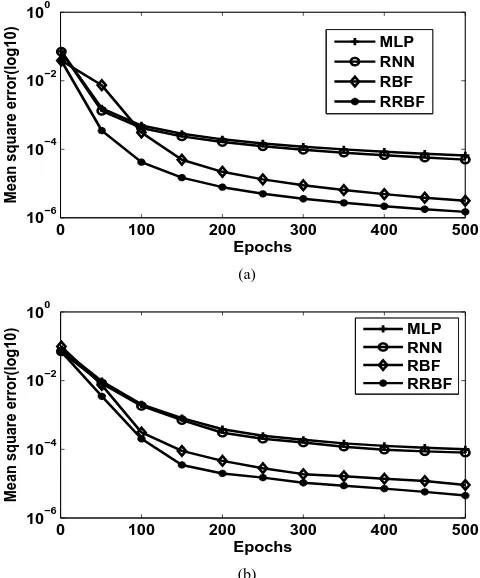
1) Convergence performance: The mean square error (MSE) of all the networks for 13-bit and 35-bit Barker codes are depicted in Fig. 3. From the figure it is evident that the RRBF based approach offers better convergence speed and very low residual error after training for 13-bit and 35-bit Barker codes as compared to all other networks.

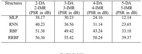
2) PSR performance: It is defined as the ratio of peak sidelobe power to the mainlobe power. After the training is over, different inputs are applied to the networks to examine PSR performance. The compressed output of different networks for 13-bit Barker code is shown in Fig. 4. The PSR values of all the networks for 13-bit and 35-bit Barker codes are listed in Table I. The table shows that the proposed

TABLE I

PSRS OBTAINED BY VARIOUS STRUCTURES

Structures 13-Bit Barker Code 35-Bit Barker Code

(PSR in dB) (PSR in dB)

MLP 42.61 40.87

RNN 45.75 44.93

RBF 60.43 56.42

RRBF 64.31 62.35

RRBF network have achieved highest PSR magnitude for both 13-bit and 35-bit Barker codes compared to all other approaches.

3) Noise performance: Noise is a random signal which interferes with the target echoes. If the noise is very high it may mask the target echo. So it is also required to examine the noise rejection ability of different networks. The inputs having different SNR ranging from 0 dB to 20 dB are applied

0 100 200 300 400 500

10−6 10−4 10−2 100

Epochs

Mean square error(log10)

MLP RNN RBF RRBF

(a)

0 100 200 300 400 500 10−6

10−4 10−2 100

Epochs

Mean square error(log10)

MLP RNN RBF RRBF

(b)

Fig. 3. Convergence graphs of different structures for (a)13-bit (b)35-bits Barker codes

to the networks and the output PSR for 13-bit and 35-bit Barker codes are listed in Tables II and III respectively. These tables show that as the SNR increases the magnitude of PSR also increases. The RRBF provides highest magnitude of PSR in all SNR values compared to those obtained by all other approaches.

TABLE II

COMPARISON OFPSRS INdBAT DIFFERENTSNRS FOR13-BITBARKER CODE

Structures SNR=0dB SNR=5dB SNR=10dB SNR=15dB SNR=20dB

MLP 14.23 28.61 36.71 38.53 39.82

RNN 17.11 32.17 38.35 40.59 41.76

RBF 35.28 45.23 50.33 55.77 57.62

RRBF 40.24 49.27 57.30 60.12 61.24

TABLE III

COMPARISON OFPSRS INdBAT DIFFERENTSNRS FOR35-BITBARKER CODE

Structures SNR=0dB SNR=5dB SNR=10dB SNR=15dB SNR=20dB

MLP 15.18 29.17 32.43 36.95 38.12

RNN 19.52 32.74 37.83 40.87 42.65

RBF 40.25 48.25 52.78 54.44 55.17

RRBF 42.25 54.69 57.47 58.60 60.57

0 5 10 15 20 25 30 0

0.2 0.4 0.6 0.8 1 1.2

Time delay

Filter response

(a)

0 5 10 15 20 25 30

0 0.2 0.4 0.6 0.8 1 1.2

Time delay

Filter response

(b)

0 5 10 15 20 25 30

−0.5 0 0.5 1 1.5

Time delay

Filter response

(c)

0 5 10 15 20 25 30

0 0.5 1

Time delay

Filter response

(d)

Fig. 4. Compressed waveforms for 13 bit Barker code using (a)MLP (b)RNN (c)RBF (d)RRBF structures

TABLE IV

COMPARISON OF RANGE RESOLUTION ABILITY FOR13-BITBARKER CODE OF TWO TARGETS HAVING SAMEIMRANDDA.

Structures 2-DA 3-DA 4-DA 5-DA

(PSR in dB) (PSR in dB) (PSR in dB) (PSR in dB)

MLP 36.53 38.52 37.32 36.16

RNN 40.24 41.23 39.23 38.78

RBF 53.32 55.25 56.76 54.23

RRBF 59.72 58.28 60.73 58.71

TABLE V

COMPARISON OF RANGE RESOLUTION ABILITY FOR35-BITBARKER CODE OF TWO TARGETS HAVING SAMEIMRANDDA.

Structures 2-DA 3-DA 4-DA 5-DA

(PSR in dB) (PSR in dB) (PSR in dB) (PSR in dB)

MLP 34.41 34.83 33.75 32.62

RNN 38.23 37.79 36.87 35.25

RBF 48.34 47.61 49.82 47.13

RRBF 53.72 55.14 54.25 53.23

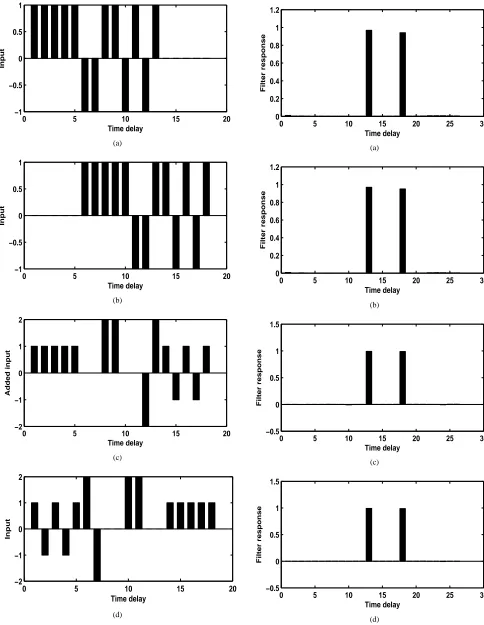
the processed echo. To compare the range resolution ability two overlapping codes of same length are considered with n-delay apart (DA) having same or different input magnitude ratio (IMR). The IMR is defined as the magnitude of first pulse train over that of the delayed pulse train. Fig. 5 shows the added input waveform of equal magnitude (IMR=1) with 5 delay apart for 13-bit Barker code. The compressed output for this input for all the network are shown in Fig. 6. In this case the PSR is calculated by taking lower value of the two mainlobes. By varying the DA from 2 to 5 the PSR for 13-bit and 35-bit Barker codes are obtained and shown in Tables IV and V respectively. In Tables VI and VII the PSR for different IMRs and DAs for all the networks are listed. From these tables it is evident that the PSR values for RRBF are the best among those offered by all other networks i.e. RRBF based pulse compression technique have best range resolution ability compared to those of other networks.

TABLE VI

COMPARISON OF RANGE RESOLUTION ABILITY FOR13-BITBARKER CODE OF TWO TARGETS HAVING DIFFERENTIMRANDDA.

Structures 2-DA 3-DA 4-DA 5-DA

2-IMR 3-IMR 4-IMR 5-IMR

(PSR in dB) (PSR in dB) (PSR in dB) (PSR in dB)

MLP 38.17 30.23 24.16 12.14

RNN 40.23 36.56 31.14 23.65

RBF 51.38 49.42 43.24 33.18

RRBF 56.36 55.42 50.24 39.37

TABLE VII

COMPARISON OF35-BITBARKER CODE FOR RANGE RESOLUTION ABILITY OF TWO TARGETS HAVING SAMEIMRANDDA

Algorithms 2-DA 3-DA 4-DA 5-DA

2-IMR 3-IMR 4-IMR 5-IMR

(PSR in dB) (PSR in dB) (PSR in dB) (PSR in dB)

MLP 34.46 27.75 21.78 14.54

RNN 39.44 33.23 26.74 20.68

RBF 47.77 45.24 38.21 25.23

0 5 10 15 20 −1

−0.5 0 0.5 1

Time delay

Input

(a)

0 5 10 15 20

−1 −0.5 0 0.5 1

Time delay

Input

(b)

0 5 10 15 20

−2 −1 0 1 2

Time delay

Added input

(c)

0 5 10 15 20

−2 −1 0 1 2

Time delay

Input

(d)

Fig. 5. Input waveform on addition of two 5-DA 13-bit Barker sequence having same magnitude (a)Left shift (b)Right shift (c)Added waveform (d)Waveform after flip about the vertical axis

0 5 10 15 20 25 30

0 0.2 0.4 0.6 0.8 1 1.2

Time delay

Filter response

(a)

0 5 10 15 20 25 30

0 0.2 0.4 0.6 0.8 1 1.2

Time delay

Filter response

(b)

0 5 10 15 20 25 30

−0.5 0 0.5 1 1.5

Time delay

Filter response

(c)

0 5 10 15 20 25 30

−0.5 0 0.5 1 1.5

Time delay

Filter response

(d)

TABLE VIII DOPPLER SHIFT PERFORMANCE

Structures 13-bit Barker code 35-bit Barker code

(PSR in dB) (PSR in dB)

MLP 14.35 28.34

RNN 30.93 42.36

RBF 47.45 46.42

RRBF 55.23 56.34

5) Doppler shift performance: The influence of Doppler shift should be accounted for evaluating the detection performance for a moving target. The Doppler tolerance measures the Doppler sensitivity of the pulse compression technique. The Doppler sensitivity is caused by the shifting in phase of the individual elements of the code by the target Doppler. In extreme case the phase shift across the code will be180o_{, the last subpulse in the received code is effectively} inverted. For 13-bit Barker code at extreme case the input will change from “1 1 1 1 1 -1 -1 1 1 -1 1 -1 1” to “-1 1 1 1 1 -1 -1 1 1 -1 1 -1 1”. For 13-bit and 35-bit Barker codes the extreme case Doppler shift PSR values for different types of network are listed in Table VIII. From this table it is observed that the MLP has very low Doppler tolerance and RRBF produces the best PSR value of 55.23 dB for 13-bit Barker code.

IV. CONCLUSION

In this paper the RRBF is proposed for radar pulse compression. The simulation results reveal that the performance of RRBF based pulse compression is much better than MLP, RNN and RBF based pulse compression techniques. The convergence rate of RRBF is higher than that of all other networks and it has low training error. The RRBF approach provides better PSR values in different adverse conditions such as noise and Doppler shift conditions. The range resolution ability of RRBF network is much superior than MLP, RNN and RBF networks. Although the algorithms are applied for 13-bit and 35-bit Barker codes, they can also be used for any other biphase codes.

REFERENCES

[1] Merrill I. Skolnik, Introduction to radar systems, McGraw Hill Book Company Inc.,1962.

[2] B. Zrnic, A. Zejak, A. Petrovic, and I. Simic, “Range sidelobe suppression for pulse compression radars utilizing modified RLS algorithm”, in Proc. IEEE Int. Symp. Spread Spectrum Techniques and Applications, Vol. 3, pp. 1008-1011, Sep 1998.

[3] Fu, J.S. and Xin Wu, “Sidelobe suppression using adaptive filtering techniques”, in Proc. CIE International Conference on Radar, pp.788-791, Oct. 2001.

[4] H. K. Kwan and C. K. Lee, “A neural network approach to pulse radar detection”, IEEE Trans. Aerosp. Electron. Syst., vol. 29, pp. 9-21, Jan.1993.

[5] A.Sailaja, A. K. Sahoo, G. Panda and V. Baghel, “A recurrent neural network approach to pulse radar detection”, IEEE Indicon’09, Dec.2009.

[6] D.G. Khairnar, S.N. Merchant and U.B. Desai, “Radial basis neural network for pulse radar detection”, IET Radar, Sonar&_{Navigation vol} 1, pp-8-17, Feb 2007

[7] S. V. T. Elanayar and Y. C. Shin, “Radial basis function neural network for approximation and estimation of nonlinear stochastic dynamic systems,” IEEE Trans. Neural Network, vol. 5, pp. 594-603, 1994. [8] S. R. Samantray, P. K. Dash and G. Panda , “Fault classification and

location using HS-transform and radial basis function neural network,” Electric Power Syst. Research, vol. 76, pp. 897-905, 2006.

[9] Y. J. Oyang, S. C. Hwang, Yu-Yen Ou, C.Y. Chen and Z.W. Chen, “Data classification with radial basis function networks based on a novel kernel density estimation algorithm,” IEEE Trans. Neural Netw., vol. 16, no.1, pp. 225-236, 2005.

[10] A. C. Tsoi and S. Tan, “Recurrent neural networks: A constructive algorithm and its properties,” Neurocomputing, vol. 15, pp. 309-326, 1997.

[11] G. Hardier, “Recurrent RBF networks for suspension system modeling and wear diagnosis of a damper,” IEEE World Congress on Comput. Intelligence, vol. 3, pp. 2441 - 2446, 1998.

[12] S.A. Billings and C.F. Fung, “Recurrent Radial Basis Function Networks for Adaptive Noise Cancellation,” Neural Netw., vol. 8, no. 2, pp. 273-290, 1995.

[13] R. Bambang, “Active noise cancellation using recurrent radial basis function neural networks,” Asia-Pacific Conf. on Circuits and Syst., vol 2, pp. 231-236A, 2002.

[14] R. Zemouri, D. Racoceanu and N. Zerhouni, “Recurrent radial basis function network for time-series prediction,” Engineering Applications of Artificial Intelligence, vol. 16, no. 5, pp. 453-463, 2003.