Short-Term Load Forecasting Using Artificial
Neural Network
Muhammad Buhari, Member, IAENG and Sanusi Sani Adamu
Abstract--Artificial neural network (ANN) has been used for
many years in sectors and disciplines like medical science, defence industry, robotics, electronics, economy, forecasts, etc. The learning property of ANN in solving nonlinear and complex problems called for its application to forecasting problems. This report present the development of an ANN based short-term load forecasting model for the 132/33KV sub-Station, Kano, Nigeria. The recorded daily load profile with a lead time of 1-24 hours for the year 2005 was obtained from the utility company. The Levenberg-Marquardt optimization technique which has one of the best learning rates was used as a back propagation algorithm for the Multilayer Feed Forward ANN model using MATLAB® R2008b ANN Toolbox. Experiences gained during the development of the model regarding the selection of the input variables, the ANN structure, and the training parameters are described. The forecasted next day 24 hourly peak loads are obtained based on the stationary output of the ANN with a performance Mean Squared Error (MSE) of . and compares favorably with the actual Power utility data. The results have shown that the proposed technique is robust in forecasting future load demands for the daily operational planning of power system distribution sub-stations in Nigeria.
Index Terms---Short term load forecasting, artificial neural
networks based Levenberg-Marquardt back propagation algorithm.
I. INTRODUCTION
Electric load demand is a function of weather variables and human social activities, industrial activities as well as community developmental level to mention a few [2-7]. Statistical techniques and Expert system techniques have failed to adequately address this issue [2-10]. The daily operation and planning activities of an electric utility requires the prediction of electricity demand of its customers. In general, the required load forecasts can be categorized into short-term, mid-term, and long-term forecasts. The short-term forecasts refer to hourly prediction of the load for a lead time ranging from one hour to several days out. The mid-term forecasts can either be hourly or peak load forecasts for a forecast horizon of one to several months ahead. Scheduling of fuel purchases, load flow studies or contingency analysis, and planning for energy, while the long-term forecasts refer to forecasts made for one to several years in the future. The quality of short-term hourly load forecasts has a significant impact on the economic operation of the electric utility since decisions such as economic scheduling of generating capacity, transactions such as ATC (Available Transmission Capacity) are based on these forecasts and they have significant economic consequences.
Manuscript received September 26, 2011: revised October 09, 2011 Muhammad Buhari is with Bayero University, Kano, P.M.B 3011 Kano, Nigeria, as an Assistant Lecturer, mobile: +2348065533305; [email protected]. Sanusi Sani Adamu is also with Bayero University, Kano, P.M.B 3011 Kano, Nigeria, as a senior lecturer; [email protected]
The need for accurate load forecasts will increase in the future because of the dramatic changes occurring in the structure of the utility industry due to deregulation and competition. This environment compels the utilities to operate at the highest possible efficiency, which, as indicated above, requires accurate load forecasts [1].
For decades the problem of improving the accuracy of load forecasts has been an important topic of research. Various types of load forecasting methodologies as reported in [1] have their own advantages. Load forecasting can be performed using many techniques such as regression analysis, statistical methods, artificial neural networks, genetic algorithm, fuzzy logic etc. Short Term load Forecaster (STLF) studies began at early 1960s with one of the first studies done by Heinemann et al. in 1966 which dealt with the relationship between temperature and load [10]. In 1971, a load forecasting system was developed by Lijesen and Rosing which used statistical approach [11]. In 1987, Hagan and Behr forecasted load using a time series model [9]. The time series approach assumes that the load of at any time depends mainly on previous load patterns. Like the autoregressive-moving average models [2] and spectral expansion technique [3], the regression method utilizes the tendency that the load pattern has a strong correlation to weather pattern [4, 5]. The weather sensitive portion of the load is arbitrarily extracted and modeled by a predetermined functional relationship with weather variables. The statistical methods, such as autoregressive moving average, linear regression, stochastic time series, and general exponential smoothing involves the use of hard computing techniques based on the exact model of the system and utilize linear analysis [2]. However, they have limited ability to capture non-linear and non-stationary characteristics of the hourly load series and are not adaptive to rapid load variations.
From 1990, researchers began to implement different approaches for STLF other than statistical approach. The emphasis shifted to the application of various AI techniques for STLF [7-11]. AI techniques like Neural Network (NN), Fuzzy NN (FNN), and Expert Systems [6] have been applied to deal with the non-linearity, huge data sets requirement in implementing the STLF systems and other difficulties in modelling of statistical methods used for application of STLF. Among the AI techniques available, different models of NNs have received great deal of attention by the researchers in the area of STLF due to flexibility in data modelling. In 1991 Park et al. were among the first group of researchers who chose to use the ANN approach for STLF [12]. Some group of researchers implemented STLF systems using hybrid methods. The study done by Srinivasan et al. in 1995 was an example of this kind of approach which used a model that consisted of fuzzy logic and neural network [13].
learning from training data set [3-5]. A comprehensive review of the literature on the application of NNs to the load forecasting was found in [6].Fuzzy Neural Networks (FNN) [7] and other techniques applying wavelets with NN [8] have also been tested for STLF. Due of the strong relationship between outside temperature and electric power demand (load), most STLF methods are based, at least in part, on temperature [17]. Often the performance of STLFs as reported in the literature is evaluated using actual temperatures that can only be known after the fact. However, when the STLF is actually used at a utility, these future temperatures are not known and forecasts have to be used instead. Among the ANN-based load forecasters discussed in published literature, ANNSTLF-artificial neural network short term load forecaster is the only one that is implemented at several sites and thoroughly tested under various real-world conditions [1]. An important aspect of ANNSTLF is that a single architecture with the same input-output structure can be used for modeling hourly loads of various size utilities in different regions of a country. The only customization required is the determination of some parameters of the ANN models. No other aspects of the models need to be altered [1].
This work involves the design of an ANNSTLF model for the 132/33KV substation Kano in order to obtain accurate forecasts of the load for a 24 hour period of the next day in advance by training the neural network with previous load data and daily average temperatures to produce a 24 hours load forecast which is necessary for the operational planning of the power system utility company. And in order to determine the connection weights between the neurons, the Levernberg Marquardt back-propagation algorithm available from Matlab-R2008b ANN toolbox was used. The network was trained with load data of year 2005 which was obtained from the Power utility Kano.
The paper begins with an introduction to STLF followed by a description of the designed neural network model. The paper concludes with a discussion of the results and a comparison with the actual data obtained from the power utility.
II. DESIGN OF THE NEURAL NETWORK MODEL
This section describes the step by step procedures for training the neural network to learn from the Year 2005 hourly load data and average temperatures of Kano (Table 1), in order to forecast next day's load demand. The Matlab ANN toolbox was utilized in designing the network architecture. The Multilayer Feedforward Network architecture with two layers was designed. The layers include the Hidden layer and the output layer. The input consists of daily 24 hour load data for 12 months of the year 2005 and daily average maximum temperature altogether making 25 inputs rows by 365 days. The output layer will be a day's 24 hours load forecast for the utility company. The Target data is the same as the input's daily 24 hours load data. The Transfer function used in the two layers is the log-sigmoid function for the hidden layers and the Purelin function at the output layers; this is to enable the network to be able to take care of any non-linearities in the input data and at the output, to be able to give a wide range of values. However, there is no theoretical approach to calculate the appropriate number of hidden layer nodes. This number was determined using a similar approach for training epochs i. e.
by examining the Mean squared error (MSE) over a validation set for a varying number of hidden layer nodes whereupon a number yielding the smallest error was selected. The pattern of connectivity characterizes the architecture of the network. A unit in the output layer determines its activity by following a two step procedure [14]. First, it computes the total weighted input , using the formula in equation 1.
… … … 1
Where is the activity level of the th unit in the previous layer and is the weight of the connection between the I th and the jth unit. Next, the unit calculates the activity using some function of the total weighted input. Typically we use the sigmoid function in equation 2.
… … … . 2)
Once the activities of all output units have been determined, the network computes the error E, which is defined by the expression in equation 3.
1
2 … … … . 3
Where is the activity level of the jth unit in the top layer and is the desired output of the jth unit. The Levenberg Marquardt (lm) back-propagation algorithm consists of six computational steps as described below:
1. It computes how fast the error changes as the activity of an output unit are changed. This error derivative (EA) is the difference between the actual and the desired activity (equation 4).
… … … . . 4
2. It then computes how fast the error change as the total input received by an output unit is changed. This quantity (EI) is the answer from step 1 multiplied by the rate at which the output of a unit changes as its total input is changed (equation 5).
1 … . . 5
3. It then computes how fast the error changes, as a weight on the connection into an output unit is changed. This quantity (EW) is the answer from step 2 multiplied by the activity level of the unit from which the connection emanates (equation 6).
… … . . 6)
allows back propagation to be applied to multilayer networks. When the activity of a unit in the previous layer changes, it affects the activities of all the output units to which it is connected. So to compute the overall effect on the error, we add together all these separate effects on output units. But each effect is simple to calculate. It is the answer in step 2 multiplied by the weight on the connection to that output unit (equation 7).
… … 7
By using steps 2 and 4, we can convert the EAs of one layer of units into EAs for the previous layer. This procedure can be repeated to get the EAs for as many previous layers as desired. Once the EA of a unit is known, we can use steps 2 and 3 to compute the EWs on its incoming connections.
5. It then advances to compute the H matrix (equation 8) and the gradient (equation 9). These are necessary in order to approach second-order training speed without having to compute the Hessian matrix. The performance function has the form of a sum of squares (MSE) and as such the Hessian matrix can be approximated as given in equation 8
… … … . 8)
and then the gradient can be computed using equation 9 as follows:
… … … . 9
where J is the Jacobian matrix that contains first derivatives of the network errors with respect to the weights and biases, and e is a vector of network errors. The Jacobian matrix can be computed through a standard back propagation technique that is much less complex than computing the Hessian matrix.
6. Finally, the Levenberg Marquadt- lm algorithm uses this approximation to the Hessian matrix in the following Newton-like update (equation 10).
… … 10
Where is the updated value of the network weight or bias and is the current weight or bias value. When the scalar µ is zero, this is just Newton's method, using the approximate Hessian matrix. When µ is large, this becomes gradient descent with a small step size. Newton's method is faster and more accurate near an error minimum, so the aim is to shift toward Newton's method as quickly as possible. Thus, µ is decreased after each successful step (reduction in performance function) and is increased only when a tentative step would increase the performance function. In this way, the performance function will always reduce in successive iterations of the algorithm.
III. THE NEURAL NETWORK TRAINING PROCESS
The Training goal was set at 0 so as to ensure zero tolerance to network computational errors. The transfer functions used were the log-sigmoid or tan-sigmoid in the Hidden layer neurons while the Purelin function was used in the output layer neurons so as not to constrain the output's values. The learning function used is the default steepest gradient descent method. The Levenberg-Marquardt learning function was used as it has a better learning rate compared to the other available functions in forecasting problems [18]. The training function used was the steepest gradient descent function and in some tests the steepest gradient descent method with momentum. The maximum number of epochs was set to 1000 which is the default value. Finally, the learning rate was also set to the default value and left to adjust automatically as the training made progress.
IV. DISCUSSION OF TRAINING RESULTS
This section is an explanation of the results obtained from the trained ANN model. These include the regression analysis plots between the output and target vectors, the general network error performance and the training state. After the successful completion of the training process three plots were made which include:
i. The regression plots
ii. The performance function Vs epochs plot iii. The training state plot
iv. The Forecast and Actual Data comparison Plot
Basically the input data set was divided into three: 70% was used for as training set while 15% each was used for testing and validation of the network output results. The training data set is necessary for obtaining the neural network's weight and bias values during network training. The validation data set is used to periodically test the ability of the network to generalize. Finally, the test data set is used in the evaluation of generalization error (i.e. MSE). Table 1 shows a sample of the input vectors of the 24 hourly load profiles for 365 days. Table 1 also shows a sample of the average maximum temperatures of the Kano sub-region.
i. The regression plot consists of four regression analysis plots; the first is a plot of the computed network output of the training data set Vs the target output, the second is that of validation data output Vs target output. The third is that of the Test data output set against the target output. The final plot is that of the overall network output data set Vs the target data set. All these plots try to show the co relation between the output data and the target data. They give an idea on the accuracy of the trained network will forecast since they show how well the network has learned the complex relationship of the input data.
number of iterations increased (training epochs) so did the errors reduces up to a best value of 5.84 at 1000 Epochs. This shows that the trained neural network forecast error is expected to be at about
5.84 of any input figures. This is obviously negligible and the network can be said to have successfully learned any complex and non linear relationship that was presented by the input data. iii. The training state plot will consist of three different
plots. The first plot is that of learning function Vs number of epochs. This shows the trend of the gradient values as the number of computational iterations increases. This is necessary in monitoring the manner in which the training progresses. The second plot is that of the learning rate (mu) against increasing number of epochs. This plot is essential in monitoring the rate at which the computed network error reduces during the progress of the training. The final plot here is that of the validation checks carried out automatically any time a sudden change is observed in the network gradient computation is carried out.
Finally, the trained network optimized weights for each of the two layers (hidden layer and output layer) and connected biases that gave the best network output-target data relationship were documented.
As mentioned earlier the choice of the number of hidden layer neurons, layer transfer function(s), training function, learning function, network architecture and other network and training parameters is a trial and error approach until the best set is attained. Table 2 shows a set of trial network parameters and their results. The input data used to obtain the tabulated results is a two year 24 hourly load data. The target data is the same as the input data set but without the average maximum daily temperatures. Also Table 2 shows that the higher the number of hidden neurons the better the MSE performance result. Due to the random nature of the input vectors the learning duration was much longer and better MSE performance was recorded when the log-sigmoid function was used in the Hidden layer neurons compared to when the tan-sigmoid transfer function was used in the network architectures. This may be attributed to the output values of the transfer function i. e. it can take on any value between plus and minus infinity, and squashes the output into the range 0 to 1. It was also observed that the network converged faster with better performance whenever the training was carried out with a larger data set as shown in the Table 2.
Furthermore, the data set is not pattern oriented because of the unavailability of enough power for distribution to consumers. The main reason is that the power demand of the Kano sub-region far exceeds the supply. The cases of special days like public holidays and festivities had little impact on the training process because of the peculiarity of the pattern of the data set.
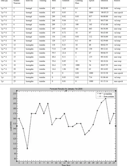
V. COMPARISON OF SIMULATED RESULTS
The simulated results of the developed model were found to be exactly the same as those obtained from the Power Utility with a performance error of5.84 , Figure 7 shows the Comparison between actual and forecast loads for 1st January, 2005 and Table 3 shows a comparison between the
actual data obtained from Power utility which is very close to the results obtained from the trained neural network model output data sets.
VI. CONCLUSIONS
A load forecasting model was designed using Matlab R2008b ANN Toolbox. The implementation of the network architecture, training of the Neural Network and simulation of test results were all successful with a very high degree of accuracy resulting into 24 hourly load output. A set of optimized weights and the associated biases after training the network from load data obtained from the power utility company were also obtained. The accuracy of the forecasts was verified by comparing the simulated outputs from the network with obtained results from the utility company. Several networks architectures were trained and simulated before arriving at the best Mean squared error performance
of 5.84 .
REFERENCES
[1] Khotanzad, A., Afkhami-Rohani, R., and Maratukulam, D., ANNSTLFArtificial neural network shortterm load forecaster-generation three, IEEE Trans. on Power Syst., 13, 4, 1413–1422, November, 1998.
[2] I. Moghram and S. Rahman, “Analysis and evaluation of five short termload forecasting techniques,” IEEE Trans. Power Syst., vol. 4, no. 4, pp. 1484–1491, Nov. 1989.
[3] C.N. Lu, H.T. Wu, and S. Vemuri, “Neural network based short term load forecasting,” IEEE Trans. Power Syst., vol. 8, no. 1, pp. 336– 342, Feb. 1993.
[4] J.W. Taylor and R. Buizza, “Neural network load forecasting with weather ensemble predictions,” IEEE Trans. Power Syst., vol. 17, no. 3, pp. 626–632, Aug. 2002.
[5] P. Mandal, T. Senjyu, N. Urasaki, and T. Funabashi, “A neural network based several-hour-ahead electric load forecasting using similar days approach,” Int. Journal. of Electric Power and Energy System, vol. 28, no. 6, pp. 367–373, July 2006.
[6] H.S. Hippert, C.E. Pedreira, and R.C. Souza, “Neural networks for short term load forecasting: A review and evaluation,” IEEE Trans. Power Syst., vol. 16, no. 1, pp. 44–55, Feb. 2001.
[7] A.G. Bakirtzis, J.B. Theocharis, S.J. Kiartzis, and K.J. Satsois, “Short term load forecasting using fuzzy neural networks” IEEE Trans. Power Syst., vol. 10, no. 3, pp. 1518–1524, Aug. 1995.
[8] J. Rocha Reis and A.P. Alves da Silva, “Feature extraction via multiresolution analysis for short-term load forecasting,” IEEE Trans. Power Systems, vol. 20, no. 1, pp. 189–198, Feb. 2005.
[9] M. T. Hagan, S. M. Behr. "The time series approach to short term load forecasting", IEEE Transactions on Power Systems, vol.2, no.3, pp.785-791, Aug. 1987
[10] G. T. Heinemann, D. A. Nordmian, E. C. Plant. "The relationship between summer weather and summer loads - a regression analysis",
IEEE Transactions on Power Apparatus and Systems, vol.PAS-85,
no.11, pp.1144-1154, Nov. 1966.
[11] D.P. Lijesen, J. Rosing. "Adaptive forecasting of hourly loads based on load measurements and weather information'', IEEE Transactions
on Power Apparatus and Systems, vol.PAS-90, no.4, pp.1757-1767,
July 1971
[12] D. C. Park, M. A. El-Sharkawi, R. J. Marks II, L. E. Atlas, M. J. Damborg. "Electric load forecasting using an artificial neural network ", IEEE Transactions on Power Systems, Vol. 6, no. 2, pp. 442-449, May 1991.
[13] D. Srinivasan, S. S. Tan, C. S. Cheng, Eng Kiat Chan. ''Parallel neural network-fuzzy expert system strategy for short-term load forecasting: system implementation and performance evaluation", IEEE
Transactions on Power Systems, vol.14, no.3, pp.1100-1106, Aug.
1999.
[15] M. Aydinalp-Koksal, A new approach for modeling of residential
energy consumption, VDM Verlag Dr. Muller Aktiengesselschaft &
Co.Kg, Pg 9-19, (2008).
[16] L. V Fausett. Fundamentals of Neural Networks, Prentice-Hall Englewood Cliffs, (1994)
[17] Khotanzad, A., Davis, M.H., Abaye, A., and Martukulam, D.J., An artificial neural network hourly temperature forecaster with applications in load forecasting, IEEE Trans. PWRS, 11, 2, 870-876, May 1996.
[18] HowardDemuth, Mark Beale, Matlab Neural Network Users Guide 4 [19]''Average monthly Maximum and Minimum temperatures for Kano.”
BBC Weather | Kano Accessed: 26 February 2011.
Table 1: 132/33KV Power Utility Substation, Kano daily Load Profile data Set for 2005
January (sample data)
Sat Sun Mon Tue Wed Thu Fri
Time 1st 2nd 3rd 4th 5th 6th 7th
1:00 AM 160 160 160 158 120 130 130
2:00 AM 140 160 160 140 126 120 190
3:00 AM 100 160 160 140 150 130 160
4:00 AM 170 156 166 156 150 140 120
5:00 AM 170 168 182 140 160 150 140
6:00 AM 190 176 180 184 144 140 180
7:00 AM 170 152 202 160 100 150 126
8:00 AM 190 180 240 180 136 120 100
9:00 AM 148 196 160 144 120 130 100
10:00 AM 160 180 170 126 144 100 100
11:00 AM 160 180 110 126 160 180 100
12:00 PM 170 170 150 110 150 0 124
1:00 PM 144 140 170 130 120 120 124
2:00 PM 144 160 170 124 120 130 124
3:00 PM 150 160 150 130 130 180 170
4:00 PM 150 160 150 130 120 120 126
5:00 PM 128 168 164 120 130 132 126
6:00 PM 136 180 140 170 130 128 180
7:00 PM 148 174 140 156 160 160 80
8:00 PM 176 180 164 152 160 170 120
9:00 PM 192 204 174 168 170 166 110
10:00 PM 200 192 156 156 170 140 150
11:00 PM 150 180 156 170 130 140 164
12:00 AM 170 168 152 164 130 126 172
[image:5.595.71.550.222.712.2]Average Temp. 18 18 18 18 18 18 18
Table 3: Simulation Results Comparison Table
January Comparison Sample
Time Sat Sat Sun Sun Mon Mon
1st 1st 2nd 2nd 3rd 3rd
1:00 AM 160.00 160.00 160.01 160.00 159.96 160.00
2:00 AM 140.00 140.00 160.00 160.00 159.96 160.00
3:00 AM 100.00 100.00 160.00 160.00 159.96 160.00
4:00 AM 170.00 170.00 156.01 156.00 165.98 166.00
5:00 AM 170.00 170.00 168.00 168.00 181.99 182.00
6:00 AM 190.00 190.00 176.00 176.00 179.97 180.00
7:00 AM 170.00 170.00 152.00 152.00 201.96 202.00
8:00 AM 190.00 190.00 180.00 180.00 239.95 240.00
9:00 AM 148.00 148.00 196.00 196.00 159.98 160.00
10:00 AM 160.00 160.00 180.00 180.00 170.01 170.00
11:00 AM 160.00 160.00 180.00 180.00 110.02 110.00
12:00 PM 170.00 170.00 170.00 170.00 149.99 150.00
1:00 PM 144.00 144.00 140.00 140.00 169.97 170.00
2:00 PM 144.00 144.00 160.00 160.00 169.98 170.00
3:00 PM 150.00 150.00 160.00 160.00 149.99 150.00
4:00 PM 149.99 150.00 160.01 160.00 150.01 150.00
5:00 PM 128.00 128.00 168.00 168.00 163.96 164.00
6:00 PM 136.00 136.00 180.00 180.00 139.97 140.00
7:00 PM 148.00 148.00 174.00 174.00 139.98 140.00
8:00 PM 176.00 176.00 180.01 180.00 163.95 164.00
9:00 PM 192.00 192.00 204.00 204.00 173.97 174.00
10:00 PM 200.00 200.00 192.00 192.00 155.95 156.00
11:00 PM 150.01 150.00 180.00 180.00 155.96 156.00
Table 2: Training Results Sample (2-layers of Logsig and purelin function neural network)
Data qty Hidden Neurons
learn fnc Training MSE Gradient Learning Rate
Epoch Duration Reason
1yr * 4 2 learngd trainlm 452 18.5 0.1 49 00:20:00 val stop
1yr * 4 3 learngd trainlm 455 0.03 0 1000 00:05:35 max epoch
1yr * 4 4 learngd trainlm 289 0.02 0.01 837 06:00:00 user stop
1yr * 4 5 learngd trainlm 248 9.04 0.1 22 00:57:00 val stop
1yr * 4 6 learngd trainlm 209 1.23 100 143 07:41:00 val stop
1yr * 4 7 learngd trainlm 187 0.03 0.1 463 06:56:00 user stop
1yr * 4 8 learngd trainlm 159 0.72 10 87 06:43:00 val stop
1yr * 4 9 learngd trainlm 136 2.02 0.01 112 08:54:00 user stop
1yr * 4 10 learngd trainlm 120 12.7 0.1 40 02:59:00 val stop
1yr * 4 12 learngdm trainlm 118 0.21 10 40 00:02:55 val stop
1yr * 4 13 learngdm trainlm 71.8 1.69 10 130 00:12:41 val stop
1yr * 4 14 learngdm trainlm 59.5 22.4 0 47 00:04:55 val stop
1yr * 4 15 learngdm trainlm 48.4 0.11 1 135 00:16:02 user stop
1yr * 4 16 learngdm trainlm 39.4 0.05 10 74 00:10:26 user stop
1yr * 4 18 learngdm trainlm 26.4 3.59 1000 54 00:07:59 user stop
1yr * 4 20 learngdm trainlm 14.4 1.06 100 63 00:14:02 user stop
1yr * 4 25 learngdm trainlm 0 0 0.01 1000 03:52:38 max epoch
1yr 25 learngdm trainlm 0 0.03 0.01 714 01:06:44 val stop
1yr 25 learngdm trainlm 0 0.01 0 1000 01:15:16 max epoch
Figure 7: Comparison Plot between actual and forecast loads for 1st January, 2005
[image:6.595.43.552.78.744.2]