Learning Entailment Relations by Global Graph Structure Optimization

Graph Structure Optimization

Jonathan Berant

Ido Dagan

Jacob Goldberger

Identifying entailment relations between predicates is an important part of applied semantic inference. In this article we propose a global inference algorithm that learns such entailment rules. First, we define a graph structure over predicates that represents entailment relations as directed edges. Then, we use a global transitivity constraint on the graph to learn the optimal set of edges, formulating the optimization problem as an Integer Linear Program. The algorithm is applied in a setting where, given a target concept, the algorithm learns on the fly all entailment rules between predicates that co-occur with this concept. Results show that our global algorithm improves performance over baseline algorithms by more than 10%.

1. Introduction

TheTextual Entailment (TE) paradigm is a generic framework for applied semantic inference. The objective of TE is to recognize whether a target textual meaning can be inferred from another given text. For example, a question answering system has to recognize that alcohol affects blood pressure is inferred from the text alcohol reduces blood pressureto answer the questionWhat affects blood pressure?In the TE framework, entailment is defined as a directional relationship between pairs of text expressions, denoted byT, the entailing text, andH, the entailed hypothesis. The textTis said to entail the hypothesisHif, typically, a human readingTwould infer thatHis most likely true (Dagan et al. 2009).

TE systems require extensive knowledge of entailment patterns, often captured as entailment rules—rules that specify a directional inference relation between two text fragments (when the rule is bidirectional this is known asparaphrasing). A common type of text fragment is aproposition, which is a simple natural language expression that contains apredicate andarguments (such asalcohol affects blood pressure), where the predicate denotes some semantic relation between theconceptsthat are expressed

∗ Tel-Aviv University, P.O. Box 39040, Tel-Aviv, 69978, Israel. E-mail:[email protected].

∗∗ Bar-Ilan University, Ramat-Gan, 52900, Israel. E-mail:[email protected].

† Bar-Ilan University, Ramat-Gan, 52900, Israel. E-mail:[email protected].

by the arguments. One important type of entailment rule specifies entailment between propositional templates, that is, propositions where the arguments are possibly re-placed by variables. A rule corresponding to the aforementioned example may beX reduce blood pressure →X affect blood pressure. Because facts and knowledge are mostly expressed by propositions, such entailment rules are central to the TE task. This has led to active research on broad-scale acquisition of entailment rules for predicates (Lin and Pantel 2001; Sekine 2005; Szpektor and Dagan 2008; Yates and Etzioni 2009; Schoenmackers et al. 2010).

Previous work has focused on learning each entailment rule in isolation. It is clear, however, that there are interactions between rules. A prominent phenomenon is that entailment is inherently a transitive relation, and thus the rulesX→YandY→Zimply the ruleX→Z.1In this article we take advantage of these global interactions to improve entailment rule learning.

After reviewing relevant background (Section 2), we describe a structure termed anentailment graphthat models entailment relations between propositional templates (Section 3). Next, we motivate and discuss a specific type of entailment graph, termed a focused entailment graph, where atarget conceptinstantiates one of the arguments of all propositional templates. For example, a focused entailment graph about the target conceptnauseamight specify the entailment relations between propositional templates likeX induce nausea,X prevent nausea, andnausea is a symptom of X.

In the core section of the article, we present an algorithm that uses a global approach to learn the entailment relations, which comprise the edges of focused entailment graphs (Section 4). We define a global objective function and look for the graph that maximizes that function given scores provided by a local entailment classifier and a global transitivity constraint. The optimization problem is formulated as anInteger Linear Program (ILP) and is solved with an ILP solver, which leads to an optimal solution with respect to the global function. In Section 5 we demonstrate that this algorithm outperforms by 12–13% methods that utilize only local information as well as methods that employ a greedy optimization algorithm (Snow, Jurafsky, and Ng 2006) rather than an ILP solver.

The article also includes a comprehensive investigation of the algorithm and its components. First, we perform manual comparison between our algorithm and the baselines and analyze the reasons for the improvement in performance (Sections 5.3.1 and 5.3.2). Then, we analyze the errors made by the algorithm against manually pre-pared gold-standard graphs and compare them to the baselines (Section 5.4). Last, we perform a series of experiments in which we investigate the local entailment classifier and specifically experiment with various sets of features (Section 6). We conclude and suggest future research directions in Section 7.

This article is based on previous work (Berant, Dagan, and Goldberger 2010), while substantially expanding upon it. From a theoretical point of view, we reformulate the two ILPs previously introduced by incorporating a prior. We show a theoretical relation between the two ILPs and prove that the optimization problem tackled is NP-hard. From an empirical point of view, we conduct many new experiments that examine both the local entailment classifier as well as the global algorithm. Last, a rigorous analysis of the algorithm is performed and an extensive survey of previous work is provided.

2. Background

In this section we survey methods proposed in past literature for learning entailment rules between predicates. First, we discuss local methods that assess entailment given a pair of predicates, and then global methods that perform inference over a larger set of predicates.

2.1 Local Learning

Three types of information have primarily been utilized in the past to learn entailment rules between predicates: lexicographic methods, distributional similarity methods, and pattern-based methods.

Lexicographic methodsuse manually prepared knowledge bases that contain in-formation about semantic relations between lexical items. WordNet (Fellbaum 1998b), by far the most widely used resource, specifies relations such as hyponymy, synonymy, derivation, andentailment that can be used for semantic inference (Budanitsky and Hirst 2006). For example, if WordNet specifies thatreduceis a hyponym ofaffect, then one can infer that X reduces Y → X affects Y. WordNet has also been exploited to automatically generate a training set for a hyponym classifier (Snow, Jurafsky, and Ng 2004), and we make a similar use of WordNet in Section 4.1.

A drawback of WordNet is that it specifies semantic relations for words and terms but not for more complex expressions. For example, WordNet does not cover a complex predicate such asX causes a reduction in Y. Another drawback of WordNet is that it only supplies semantic relations between lexical items, but does not provide any information on how to map arguments of predicates. For example, WordNet specifies that there is an entailment relation between the predicatespayand buy, but does not describe the way in which arguments are mapped: ifX pays Y for Z then X buys Z from Y. Thus, using WordNet directly to derive entailment rules between predicates is possible only for semantic relations such as hyponymy and synonymy, where arguments typically preserve their syntactic positions on both sides of the rule.

Some knowledge bases try to overcome this difficulty: Nomlex (Macleod et al. 1998) is a dictionary that provides the mapping of arguments between verbs and their nominalizations and has been utilized to derive predicative entailment rules (Meyers et al. 2004; Szpektor and Dagan 2009). FrameNet (Baker, Fillmore, and Lowe 1998) is a lexicographic resource that is arranged around “frames”: Each frame corresponds to an event and includes information on the predicates and arguments relevant for that specific event supplemented with annotated examples that specify argument positions. Consequently, FrameNet was also used to derive entailment rules between predicates (Coyne and Rambow 2009; Ben Aharon, Szpektor, and Dagan 2010). Additional man-ually constructed resources for predicates include PropBank (Kingsbury, Palmer, and Marcus 2002) and VerbNet (Kipper, Dang, and Palmer 2000).

Lin and Pantel (2001) proposed an algorithm that is based on a mutual information criterion. A predicate is represented by abinary template, which is a dependency path between two arguments of a predicate where the arguments are replaced by variables. Note that in a dependency tree, a path between two arguments must pass through their common predicate. Also note that if a predicate has more than two arguments, then it is represented by more than one binary template, where each template corresponds to a different aspect of the predicate. For example, the proposition I bought a gift for her contains a predicate and three arguments, and therefore is represented by the following three binary templates:X←−−subj buys−→obj Y,X←−obj buys−−→prep for−−−−−→pcomp−n YandX←−−subj buys

prep

−−→for−−−−−→pcomp−n Y.

For each binary template Lin and Pantel compute two sets of features F_x andF_y, which are the words that instantiate the arguments Xand Y, respectively, in a large corpus. Given a template t and its feature set for the X variable Ft_x, everyfx ∈Ftx is weighted by the pointwise mutual information between the template and the feature: wt_x(fx)=log

Pr(fx|t)

Pr(fx), where the probabilities are computed using maximum likelihood

over the corpus. Given two templatesuandv, theLinmeasure (Lin 1998a) is computed for the variableXin the following manner:

Linx(u,v)=

f∈Fu x∩Fvx[w

u

x(f)+wvx(f)]

f∈Fu xw

u x(f)+

f∈Fv xw

v x(f)

(1)

The measure is computed analogously for the variable Yand the final distributional similarity score, termed DIRT, is the geometric average of the scores for the two variables:

DIRT(u,v)=

Linx(u,v)·Liny(u,v) (2)

IfDIRT(u,v) is high, this means that the templatesuandvshare many “informative” arguments and so it is possible that u→v. Note, however, that the DIRT similarity measure computes a symmetric score, which is appropriate for modeling synonymy but not entailment, an inherently directional relation.

To remedy that, Szpektor and Dagan (2008) suggested a directional distributional similarity measure. In their work, Szpektor and Dagan chose to represent predicates withunary templates, which are identical to binary templates, only they contain a pred-icate and a single argument, such as:X←−−subj buys. Szpektor and Dagan explain that unary templates are more expressive than binary templates, and that some predicates can only be encoded using unary templates. They propose that if for two unary templatesu→v, then relatively many of the features ofu should be covered by the features ofv. This is captured by the asymmetricCovermeasure suggested by Weeds and Weir (2003) (we omit the subscriptxfromFu_xandFv_xbecause in their setting there is only one argument):

Cover(u,v)=

f∈Fu∩_Fvwu(f)

f∈Fuwu(f)

(3)

The final directional score, termedBInc(Balanced Inclusion), is the geometric average of theLinmeasure and theCovermeasure:

Both Lin and Pantel as well as Szpektor and Dagan compute a similarity score for each argument separately, effectively decoupling the arguments from one another. It is clear, however, that although this alleviates sparsity problems, it disregards an impor-tant piece of information, namely, the co-occurrence of arguments. For example, if one looks at the following propositions:coffee increases blood pressure,coffee decreases fatigue, wine decreases blood pressure,wine increases fatigue, one can notice that the predicates occur with similar arguments and might mistakenly infer thatdecrease→increase. However, looking at pairs of arguments reveals that the predicates do not share a single pair of arguments.

Yates and Etzioni (2009) address this issue and propose a generative model that estimates the probability that two predicates are synonymous (synonymy is simply bidirectional entailment) by comparing pairs of arguments. They represent predicates and arguments as strings and compute for every predicate a feature vector that counts that number of times it occurs with any ordered pair of words as arguments. Their main modeling decision is to assume that two predicates are synonymous if the number of pairs of arguments they share is maximal. An earlier work by Szpektor et al. (2004) also tried to learn entailment rules between predicates by using pairs of arguments as features. They utilized an algorithm that learns new rules by searching for distributional similarity information on the Web for candidate predicates.

Pattern-based methods.Although distributional similarity measures excel at iden-tifying the existence of semantic similarity between predicates, they are often unable to discern the exact type of semantic similarity and specifically determine whether it is entailment. Pattern-based methods are used to automatically extract pairs of predicates for a specific semantic relation. Pattern-based methods identify a semantic relation between two predicates by observing that they co-occur in specific patterns in sentences. For example, from the single propositionHe scared and even startled meone might infer thatstartleis semantically stronger thanscareand thus startle→ scare. Chklovski and Pantel (2004) manually constructed a few dozen patterns and learned semantic relations between predicates by looking for these patterns on the Web. For example, the pattern X and even Yimplies thatYis stronger thanX, and the patternto X and then Yindicates thatYfollowsX. The main disadvantage of pattern-based methods is that they are based on the co-occurrence of two predicates in a single sentence in a specific pattern. These events are quite rare and require working on a very large corpus, or preferably, the Web. Pattern-based methods were mainly utilized so far to extract semantic relations between nouns, and there has been some work on automatically learning patterns for nouns (Snow, Jurafsky, and Ng 2004). Although these methods can be expanded for predicates, we are unaware of any attempt to automatically learn patterns that describe semantic relations between predicates (as opposed to the manually constructed patterns suggested by Chklovski and Pantel [2004]).

2.2 Global Learning

and Dagan 2008). Their resource makes simple use of WordNet’s global graph structure: New rules are suggested by transitively chaining graph edges, and then verified using distributional similarity measures. Effectively, this is equivalent to using the intersection of the set of rules derived by this transitive chaining and the set of rules in a distribu-tional similarity knowledge base.

The most similar work to ours is Snow, Jurafsky, and Ng’s (2006) algorithm for taxonomy induction, although it involves learning the hyponymy relation between nouns, which is a special case of entailment, rather than learning entailment between predicates. We provide here a brief review of a simplified form of this algorithm.

Snow, Jurafsky, and Ng define a taxonomyTto be a set of pairs of words, expressing the hyponymy relation between them. The notationH_uv∈Tmeans that the nounuis a hyponym of the nounvinT. They defineDto be the set of observed data over all pairs of words, and defineDuv∈Dto be the observed evidence we have in the data for the event

Huv∈T. Snow, Jurafsky, and Ng assume a model exists for inferringP(Huv∈T|Duv): the posterior probability of the eventHuv∈T, given the data. Their goal is to find the taxonomy that maximizes the likelihood of the data, that is, to find

ˆ

T=argmax T

P(D|T) (5)

Using some independence assumptions and Bayes rule, the likelihood P(D|T) is expressed:

P(D|T)=

Huv∈T

P(Huv∈T|Duv)P(Duv)

P(H_uv∈T) ·

Huv∈/T

P(Huv∈/T|Duv)P(Duv)

P(Huv∈/T)

(6)

Crucially, they demand that the taxonomy learned respects the constraint that hy-ponymy is a transitive relation. To ensure that, they propose the following greedy algorithm: At each step they go over all pairs of words (u,v) that are not in the taxonomy, and try to add the single hyponymy relationH_uv. Then, they calculate the set of relations S_uv that H_uv will add to the taxonomy due to the transitivity constraint (all of the relations H_uw, where w is a hypernym of v in the taxonomy). Last, they choose to add that set of relationsS_uvthat maximizesP(D|T) out of all the possible candidates. This iterative process stops whenP(D|T) starts dropping. Their implementation of the algorithm uses a hyponym classifier presented in an earlier work (Snow, Jurafsky, and Ng 2004) as a model forP(H_uv∈T|D_uv) and a singlesparsityparameterk= P(Huv∈/T)

P(Huv∈T). In

this article we tackle a similar problem of learning a transitive relation, but we use linear programming (Vanderbei 2008) to solve the optimization problem.

2.3 Linear Programming

ALinear Program (LP)is an optimization problem where a linear objective function is minimized (or maximized) under linear constraints.

min x∈Rd

cx (7)

such thatAx≤b

that allnlinear constraints specified by the matrixAand the vectorbare satisfied by this assignment. If the variables are forced to be integers, the problem is termed an Integer Linear Program (ILP). ILP has attracted considerable attention recently in several fields of NLP, such as semantic role labeling, summarization, and parsing (Althaus, Karamanis, and Koller 2004; Roth and Yih 2004; Riedel and Clarke 2006; Clarke and Lapata 2008; Finkel and Manning 2008; Martins, Smith, and Xing 2009). In this article we formulate the entailment graph learning problem as an ILP, which leads to an optimal solution with respect to the objective function (vs. a greedy optimization algorithm suggested by Snow, Jurafsky, and Ng [2006]). Recently, Do and Roth (2010) used ILP in a related task of learning taxonomic relations between nouns, utilizing constraints between sibling nodes and ancestor–child nodes in small graphs of three nodes.

3. Entailment Graph

In this section we define a structure termed the entailment graphthat describes the entailment relations between propositional templates (Section 3.1), and a specific type of entailment graph, termed thefocused entailment graph, that concentrates on entail-ment relations that are relevant for some pre-defined target concept (Section 3.2).

3.1 Entailment Graph: Definition and Properties

The nodes of an entailment graph arepropositional templates. A propositional tem-plate is a binary temtem-plate2where at least one of the two arguments is a variable whereas the second may be instantiated. In addition, the sense of the predicate is specified (ac-cording to some sense inventory, such as WordNet) and so each sense of a polysemous predicate corresponds to a separate template (and a separate graph node). For example,

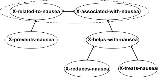
X←−−subj treats#1−→obj YandX←−−subj treats#2−→obj nauseaare propositional templates for the first and second sense of the predicatetreat, respectively. An edge (u,v) represents the fact that template u entails template v. Note that the entailment relation transcends hyponymy/troponomy. For example, the templateX is diagnosed with asthmaentails the templateX suffers from asthma, although one is not a hyponym of the other. An example of an entailment graph is given in Figure 1.

Because entailment is a transitive relation, an entailment graph istransitive, that is, if the edges (u,v) and (v,w) are in the graph, so is the edge (u,w). Note that the property of transitivity does not hold when the senses of the predicates are not specified. For example,X buys Y→X acquires YandX acquires Y→X learns Y, butX buys YX learns Y. This violation occurs because the predicateacquirehas two distinct senses in the two templates, but this distinction is lost when senses are not specified.

Transitivity implies that in each strongly connected component3 of the graph all nodes entail each other. For example, in Figure 1 the nodesX-related-to-nausea and X-associated-with-nausea form a strongly connected component. Moreover, if we merge every strongly connected component to a single node, the graph becomes a Directed Acyclic Graph (DAG), and a hierarchy of predicates can be obtained.

2 We restrict our discussion to templates with two arguments, but generalization is straightforward. 3 A strongly connected component is a subset of nodes in the graph where there is a path from any

Figure 1

A focused entailment graph. For clarity, edges that can be inferred by transitivity are omitted. The single strongly connected component is surrounded by a dashed line.

3.2 Focused Entailment Graphs

In this article we concentrate on learning a type of entailment graph, termed the focused entailment graph. Given a target concept, such as nausea, a focused entailment graph describes the entailment relations between propositional templates for which the target concept is one of the arguments (see Figure 1). Learning such entailment rules in real time for a target concept is useful in scenarios such as information retrieval and question answering, where a user specifies a query about the target concept. The need for such rules has been also motivated by Clark et al. (2007), who investigated what types of knowledge are needed to identify entailment in the context of the RTE challenge, and found that often rules that are specific to a certain concept are required. Another example for a semantic inference algorithm that is utilized in real time is provided by Do and Roth (2010), who recently described a system that, given two terms, determines the taxonomic relation between them on the fly. Last, we have recently suggested an application that uses focused entailment graphs to present information about a target concept according to a hierarchy of entailment (Berant, Dagan, and Goldberger 2010).

The benefit of learning focused entailment graphs is three-fold. First, the target concept that instantiates the propositional template usually disambiguates the predicate and hence the problem of predicate ambiguity is greatly reduced. Thus, we do not employ any form of disambiguation in this article, but assume that every node in a focused entailment graph has a single sense (we further discuss this assumption when describing the experimental setting in Section 5.1), which allows us to utilize transitivity constraints.

An additional (albeit rare) reason that might also cause violations of transitivity constraints is the notion of probabilistic entailment. Whereas troponomy rules (Fellbaum 1998a) such asX walks→X movescan be perceived as being almost always correct, rules such as X coughs→X is sick might only be true with some probability. Consequently, chaining a few probabilistic rules such as A→B, B→C, and C→D might not guarantee the correctness ofA→D. Because in focused entailment graphs the number of nodes and diameter4 are quite small (for example, in the data set we

present in Section 5 the maximal number of nodes is 26, the average number of nodes is 22.04, the maximal diameter is 5, and the average diameter is 2.44), we do not find this to be a problem in our experiments in practice.

Last, the optimization problem that we formulate is NP-hard (as we show in Sec-tion 4.2). Because the number of nodes in focused entailment graphs is rather small, a standard ILP solver is able to quickly reach the optimal solution.

To conclude, the algorithm we suggest next is applied in our experiments on focused entailment graphs. However, we believe that it is suitable for any entailment graph whose properties are similar to those of focused entailment graphs. For brevity, from now on the termentailment graphwill stand forfocused entailment graph.

4. Learning Entailment Graph Edges

In this section we present an algorithm that, given the set of propositional templates constituting the nodes of an entailment graph, learns its edges (i.e., the entailment relations between all pairs of nodes). The algorithm comprises two steps (described in Sections 4.1 and 4.2): In the first step we use a large corpus and a lexicographic resource (WordNet) to train a genericentailment classifierthat given any pair of propositional templates estimates the likelihood that one template entails the other. This generic step is performed only once, and is independent of the specific nodes of the target entailment graph whose edges we want to learn. In the second step we learn on the fly the edges of a specific target graph: Given the graph nodes, we use a global optimization approach that determines the set of edges that maximizes the probability (or score) of the entire graph. The global graph decision is determined by the given edge probabilities (or scores) supplied by the entailment classifier and by the graph constraints (transitivity and others).

4.1 Training an Entailment Classifier

We describe a procedure for learning a generic entailment classifier, which can be used to estimate the entailment likelihood for any given pair of templates. The classifier is constructed based on a corpus and a lexicographic resource (WordNet) using the following four steps:

(1) Extract a large set of propositional templates from the corpus.

(2) Use WordNet to automatically generate a training set of pairs of templates—both positive and negative examples.

(3) Represent each training set example with a feature vector of various distributional similarity scores.

(4) Train a classifier over the training set.

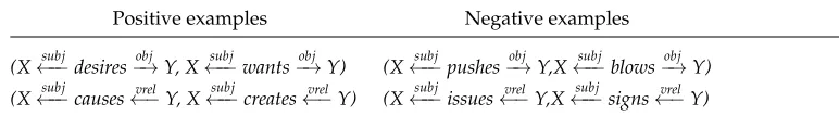
Table 1

Positive and negative examples for entailment in the training set. The direction of entailment is from the left template to the right template.

Positive examples Negative examples

(X←−−subj desires−→obj Y, X←−−subj wants−→obj Y) (X←−−subj pushes−→obj Y,X←−−subj blows−→obj Y)

(X←−−subj causes←−vrel Y, X←−−subj creates←−vrel Y) (X←−−subj issues←−vrel Y,X←−−subj signs←−vrel Y)

a simple heuristic to filter out templates that probably do not include a predicate: We omit “uni-directional” templates where the root of template has a single child, such as therapy−−→prepin−−−−→p−comppatient−→nncancer, unless one of the edges is labeled with a passive relation, such as in the template nausea ←−−vrelcharacterized←−−subjpoisoning, which contains the Minipar passive labelvrel.5Last, the arguments are replaced by variables, resulting in propositional templates such as X←−−subj affect−→obj Y. The lexical items that remain in the template after replacing the arguments by variables are termedpredicate words.

(2)Training set generation. WordNet is used to automatically generate a training set of positive (entailing) and negative (non-entailing) template pairs. LetTbe the set of propositional templates extracted from the corpus. For eacht_i∈Twith two variables and a single predicate wordw, we extract from WordNet the setHof direct hypernyms (distance of one in WordNet) and synonyms ofw. For everyh∈H, we generate a new template tjfromti by replacingwwith h. Iftj∈T, we consider (ti,tj) to be a positive example. Negative examples are generated analogously, only considering direct co-hyponyms of w, which are direct hyponyms of direct hypernyms of w that are not synonymous tow. It has been shown in past work that in most cases co-hyponym terms do not entail one another (Mirkin, Dagan, and Gefet 2006). A few examples for positive and negative training examples are given in Table 1.

This generation method is similar to the “distant supervision” method proposed by Snow, Jurafsky, and Ng (2004) for training a noun hypernym classifier. It differs in some important aspects, however: First, Snow, Jurafsky, and Ng consider a positive example to be any Wordnet hypernym, irrespective of the distance, whereas we look only at direct hypernyms. This is because predicates are mainly verbs and precision drops quickly when looking at verb hypernyms in WordNet at a longer distance. Second, Snow, Jurafsky, and Ng generate negative examples by looking at any two nouns where one is not the hypernym of the other. In the spirit of “contrastive estimation” (Smith and Eisner 2005), we prefer to generate negative examples that are “hard,” that is, negative examples that, although not entailing, are still semantically similar to positive examples and thus focus the classifier’s attention on determining the boundary of the entailment class. Last, we use a balanced number of positive and negative examples, because classifiers tend to perform poorly on the minority class when trained on imbalanced data (Van Hulse, Khoshgoftaar, and Napolitano 2007; Nikulin 2008).

(3)Distributional similarity representation.We aim to train a classifier that for an input template pair (t1,t2) determines whethert1entailst2. Our approach is to represent

a template pair by a feature vector where each coordinate is a different distributional similarity score for the pair of templates. The different distributional similarity scores

are obtained by utilizing various distributional similarity algorithms that differ in one or more of their characteristics. In this way we hope to combine the various methods proposed in the past for measuring distributional similarity. The distributional similar-ity algorithms we employ vary in one or more of the following dimensions: the way the predicate is represented, the way the features are represented, and the function used to measure similarity between the feature representations of the two templates.

Predicate representation. As mentioned, we represent predicates over dependency tree structures. However, some distributional similarity algorithms measure similarity between binary templates directly (Lin and Pantel 2001; Szpektor et al. 2004; Bhagat, Pantel, and Hovy 2007; Yates and Etzioni 2009), whereas others decompose binary templates into two unary templates, estimate similarity between two pairs of unary templates, and combine the two scores into a single score (Szpektor and Dagan 2008).

Feature representation.The features of a template are some function of the terms that instantiated the argument variables in a corpus. Two representations that are used in our experiments are derived from an ontology that maps natural language phrases to semantic identifiers (see Section 5). Another variant occurs when using binary tem-plates: a template may be represented by a pair of feature vectors, one for each variable as in the DIRT algorithm (Lin and Pantel 2001), or by a single vector, where features represent pairs of instantiations (Szpektor et al. 2004; Yates and Etzioni 2009). The former variant reduces sparsity problems, whereas Yates and Etzioni showed the latter is more informative and performs favorably on their data.

Similarity function.We consider two similarity functions: The symmetric Lin(Lin and Pantel 2001) similarity measure, and the directional BInc (Szpektor and Dagan 2008) similarity measure, reviewed in Section 2. Thus, information about the direction of entailment is provided by theBIncmeasure.

We compute for any pair of templates (t₁,t₂) 12 distributional similarity scores using all possible combinations of the aforementioned dimensions. These scores are then used as 12 features representing the pair (t1,t2). (A full description of the features is given in

Section 5.) This is reminiscent of Connor and Roth (2007), who used the output of unsu-pervised classifiers as features for a suunsu-pervised classifier in a verb disambiguation task. (4)Training a classifierTwo types of classifiers may be trained in our scheme over the training set: margin classifiers (such as SVM) and probabilistic classifiers. Given a pair of templates (u,v) and their feature vectorFuv, we denote by an indicator variable

Iuv the event that u entails v. A margin classifier estimates a score Suv for the event

Iuv=1, which indicates the positive or negative distance of the feature vectorFuvfrom the separating hyperplane. A probabilistic classifier provides the posterior probability Puv=P(Iuv=1|Fuv).

4.2 Global Learning of Edges

In this step we get a set of propositional templates as input, and we would like to learn all of the entailment relations between these propositional templates. For every pair of templates we can compute the distributional similarity features and get a score from the trained entailment classifier. Once all the scores are calculated we try to find the optimal graph—that is, the best set of edges over the propositional templates. Thus, in this scenario the input is the nodes of the graph and the output are the edges.

entailment classifier in our case), we want to learn the directed graphG=(V,E), where E={(u,v)|Iuv=1}, by solving the following ILP over the variablesIuv:

ˆ

G=argmax G

u=v

f(u,v)·I_uv (8)

s.t.∀u,v,w∈VIuv+Ivw−Iuw≤1 (9)

∀u,v∈AyesIuv=1 (10)

∀u,v∈AnoIuv=0 (11)

∀u=vIuv∈ {0, 1} (12)

The objective function in Equation (8) is simply a sum over the weights of the graph edges. The global constraint is given in Equation (9) and states that the graph must respect transitivity. This constraint is equivalent to the one suggested by Finkel and Manning (2008) in a coreference resolution task, except that the edges of our graph are directed. The constraints in Equations (10) and (11) state that for a few node pairs, defined by the setsAyesandAno, respectively, we have prior knowledge that one node does or does not entail the other node. Note that if (u,v)∈Ano, then due to transitivity there must be no path in the graph fromutov, which rules out additional edge combi-nations. We elaborate on how the setsA_yesandA_noare computed in our experiments in Section 5. Altogether, this Integer Linear Program containsO(|V|2) variables andO(|V|3) constraints, and can be solved using state-of-the-art optimization packages.

A theoretical aspect of this optimization problem is that it is NP-hard. We can phrase it as a decision problem in the following manner: GivenV, f, and a threshold k, we wish to know if there is a set of edgesEthat respects transitivity and

(u,v)∈E

f(u,v)≥k.

Yannakakis (1978) has shown that the simpler problem of finding in a graph G= (V,E) a subset of edgesA⊆Ethat respects transitivity and|A| ≥kis NP-hard. Thus, we can conclude that our optimization problem is also NP-hard by the trivial poly-nomial reduction defining the functionfthat assigns the score 0 for node pairs (u,v)∈/E and the score 1 for node pairs (u,v)∈E. Because the decision problem is NP-hard, it is clear that the corresponding maximization problem is also NP-hard. Thus, obtaining a solution using ILP is quite reasonable and in our experiments also proves to be efficient (Section 5).

Next, we describe two ways of obtaining the weighting functionf, depending on the type of entailment classifier we prefer to train.

4.2.1 Score-Based Weighting Function. In this case, we assume that we choose to train a margin entailment classifier estimating the score Suv (a positive score if the classifier predicts entailment, and a negative score otherwise) and define_{f score}(u,v)=Suv−λ. This gives rise to the following objective function:

ˆ

Gscore=argmax G

u=v

(Suv−λ)·Iuv=argmax G

 

u=v

Suv·Iuv



₋λ· |E| (13)

Suv> λ, or in other words to “push” the separating hyperplane towards the positive half space byλ. Note that the constantλis a parameter that needs to be estimated and we discuss ways of estimating it in Section 5.2.

4.2.2 Probabilistic Weighting Function. In this case, we assume that we choose to train a probabilistic entailment classifier. Recall that Iuv is an indicator variable denoting whetheruentailsv, thatFuvis the feature vector for the pair of templatesuandv, and de-fineFto be the set of feature vectors for all pairs of templates in the graph. The classifier estimates the posterior probability of an edge given its features:Puv=P(Iuv=1|Fuv), and we would like to look for the graph Gthat maximizes the posterior probability P(G|F). In Appendix A we specify some simplifying independence assumptions under which this graph maximizes the following linear objective function:

ˆ

Gprob=argmax G

u=v

(log Puv 1−Puv

+logη)·Iuv=argmax G

u=v

log Puv 1−Puv ·

Iuv+logη· |E|

(14)

whereη= P(Iuv=1)

P(Iuv=0) is the prior odds ratio for an edge in the graph, which needs to be

estimated in some manner. Thus, the weighting function is defined by _fprob(u,v)= log Puv

1−Puv+logη.

Both the score-based and the probabilistic objective functions obtained are quite similar: Both contain a weighted sum over the edges and a regularization component reflecting the sparsity of the graph. Next, we show that we can provide a probabilistic interpretation for our score-based function (under certain conditions), which will allow us to use a margin classifier and interpret its output probabilistically.

4.2.3 Probabilistic Interpretation of Score-Based Weighting Function.We would like to use the scoreSuv, which is bounded in (∞,−∞), and derive from it a probabilityPuv. To that end we projectSuv onto (0, 1) using the sigmoid function, and definePuv in the following manner:

P_uv= 1

1+exp(−S_uv) (15)

Note that under this definition the log probability ratio is equal to the inverse of the sigmoid function:

log Puv 1−Puv

=log

1 1+exp(−Suv)

exp(−Suv) 1+exp(−Suv)

=log 1 exp(−Suv)

=Suv (16)

Therefore, when we derivePuv from Suv with the sigmoid function, we can rewrite ˆ

Gprobas:

ˆ

Gprob=argmax G

u=v

Suv·Iuv+logη· |E|=Gscoreˆ (17)

Moreover, assume that the score Suv is computed as a linear combination over n features (such as a linear-kernel SVM), that is, Suv=

n

i=1Siuv·αi, whereSiuv denotes feature values and α_i denotes feature weights. In this case, the projected probability acquires the standard form of a logistic classifier:

Puv= 1

1+exp(− n

i=1

Si_uv·α_i)

(18)

Hence, we can train the weights αi using a margin classifier and interpret the output of the classifier probabilistically, as we do with a logistic classifier. In our experiments in Section 5 we indeed use a linear-kernel SVM to train the weights α_i and then we can interchangeably interpret the resulting ILP as either score-based or probabilistic optimization.

4.2.4 Comparison to Snow, Jurafsky, and Ng (2006).Our work resembles Snow, Jurafsky, and Ng’s work in that both try to learn graph edges given a transitivity constraint. There are two key differences in the model and in the optimization algorithm, however. First, they employ a greedy optimization algorithm that incrementally adds hyponyms to a large taxonomy (WordNet), whereas we simultaneously learn all edges using a global optimization method, which is more sound and powerful theoretically, and leads to the optimal solution. Second, Snow, Jurafsky, and Ng’s model attempts to determine the graph that maximizes the likelihoodP(F|G) and not the posteriorP(G|F). If we cast their objective function as an ILP we get a formulation that is almost identical to ours, only containing theinverseprior odds ratio log1

η=−logηrather than the prior odds

ratio as the regularization term (cf. Section 2):

ˆ

GSnow=argmax G

u=v

log Puv (1−Puv)·

Iuv−logη· |E| (19)

This difference is insignificant whenη∼1, or whenηis tuned empirically for optimal performance on a development set. If, however,ηis statistically estimated, this might cause unwarranted results: Their model will favor dense graphs when the prior odds ratio is low (η <1 orP(Iuv=1)<0.5), and sparse graphs when the prior odds ratio is high (η >1 orP(Iuv=1)>0.5), which is counterintuitive. Our model does not suffer from this shortcoming because it optimizes the posterior rather than the likelihood. In Section 5 we show that our algorithm significantly outperforms the algorithm presented by Snow, Jurafsky, and Ng.

5. Experimental Evaluation

This section presents an evaluation and analysis of our algorithm.

5.1 Experimental Setting

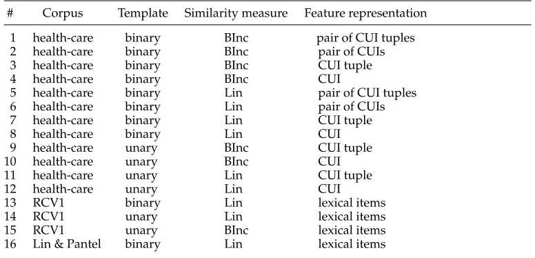
Table 2

The similarity score features used to represent pairs of templates. The columns specify the corpus over which the similarity score was computed, the template representation, the similarity measure employed, and the feature representation (as described in Section 4.1).

# Corpus Template Similarity measure Feature representation

1 health-care binary BInc pair of CUI tuples 2 health-care binary BInc pair of CUIs 3 health-care binary BInc CUI tuple 4 health-care binary BInc CUI

5 health-care binary Lin pair of CUI tuples 6 health-care binary Lin pair of CUIs 7 health-care binary Lin CUI tuple 8 health-care binary Lin CUI 9 health-care unary BInc CUI tuple 10 health-care unary BInc CUI 11 health-care unary Lin CUI tuple

12 health-care unary Lin CUI

13 RCV1 binary Lin lexical items

14 RCV1 unary Lin lexical items

15 RCV1 unary BInc lexical items 16 Lin & Pantel binary Lin lexical items

word tokens. We used the Unified Medical Language System (UMLS)6 to annotate medical concepts in the corpus. The UMLS is a database that maps natural language phrases to over one million concept identifiers in the health-care domain (termed CUIs). We annotated all nouns and noun phrases that are in the UMLS with their (possibly multiple) CUIs. We now provide the details of training an entailment classifier as explained in Section 4.1.

We extracted all templates from the corpus where both argument instantiations are medical concepts, that is, annotated with a CUI (∼50,000 templates). This was done to increase the likelihood that the extracted templates are related to the health-care domain and reduce problems of ambiguity.

As explained in Section 4.1, a pair of templates constitutes an input example for the entailment classifier, and should be represented by a set of features. The features we used were different distributional similarity scores for the pair of templates, as summarized in Table 2. Twelve distributional similarity measures were computed over the health-care corpus using the aforementioned variations (Section 4.1), where two feature representations were considered: in the UMLS each natural language phrase may be mapped not to a single CUI, but to a tuple of CUIs. Therefore, in the first representation, each feature vector coordinate counts the number of times a tuple of CUIs was mapped to the term instantiating the template argument, and in the second representation it counts the number of times each single CUI was one of the CUIs mapped to the term instantiating the template argument. In addition, we obtained the original template similarity lists learned by Lin and Pantel (2001), and had available three distributional similarity measures learned by Szpektor and Dagan (2008), over the RCV1 corpus,7 as detailed in Table 2. Thus, each pair of templates is represented by a total of 16 distributional similarity scores.

6 http://www.nlm.nih.gov/research/umls.

We automatically generated a balanced training set of 20,144 examples using Word-Net and the procedure described in Section 4.1, and trained the entailment classifier with SVMperf (Joachims 2005). We use the trained classifier to obtain estimates forPuv and Suv, given that the score-based and probabilistic scoring functions are equivalent (cf. Section 4.2.3).

To evaluate the performance of our algorithm, we manually constructed gold-standard entailment graphs. First, 23 medical target concepts, representing typical top-ics of interest in the medical domain, were manually selected from a (longer) list of the most frequent concepts in the health-care corpus. The 23 target concepts are:alcohol, asthma,biopsy,brain,cancer,CDC,chemotherapy,chest,cough,diarrhea,FDA,headache,HIV, HPV,lungs,mouth,muscle,nausea,OSHA,salmonella,seizure,smoking, andx-ray. For each concept, we wish to learn a focused entailment graph (cf. Figure 1). Thus, the nodes of each graph were defined by extracting all propositional templates in which the corre-sponding target concept instantiated an argument at least K(=3) times in the health-care corpus (average number of graph nodes = 22.04, std = 3.66, max = 26, min = 13).

Ten medical students were given the nodes of each graph (propositional templates) and constructed the gold standard of graph edges using a Web interface. We gave an oral explanation of the annotation process to each student, and the first two graphs annotated by every student were considered part of the annotator training phase and were discarded. The annotators were able to select every propositional template and observe all of the instantiations of that template in our health-care corpus. For example, selecting the templateX helps with nauseamight show the propositionsrelaxation helps with nausea,acupuncture helps with nausea, andNabilone helps with nausea. The concept ofentailmentwas explained under the framework of TE (Dagan et al. 2009), that is, the templatet₁entails the templatet₂if given that the instantiation oft₁with some concept is true then the instantiation oft₂with the same concept is most likely true.

As explained in Section 3.2, we did not perform any disambiguation because a target concept disambiguates the propositional templates in focused entailment graphs. In practice, cases of ambiguity were very rare, except for a single scenario where in templates such asX treats asthma, annotators were unclear whetherXis a type of doctor or a type of drug. The annotators were instructed in such cases to select the template, read the instantiations of the template in the corpus, and choose the sense that is most prevalent in the corpus. This instruction was applicable to all cases of ambiguity.

Each concept graph was annotated by two students. Following the current recog-nizing TE (RTE) practice (Bentivogli et al. 2009), after initial annotation the two students met for a reconciliation phase. They worked to reach an agreement on differences and corrected their graphs. Inter-annotator agreement was calculated using the kappa statis-tic (Siegel and Castellan 1988) both before (κ=0.59) and after (κ=0.9) reconciliation. Each learned graph was evaluated against the two reconciliated graphs.

Summing the number of possible edges over all 23 concept graphs we get 10,364 possible edges, of which 882 on average were included by the annotators (averaging over the two gold-standard annotations for each graph). The concept graphs were randomly split into a development set (11 concepts) and a test set (12 concepts).

We used the lpsolve8 package to learn the edges of the graphs. This package ef-ficiently solves the model without imposing integer restrictions9 and then uses the branch-and-bound method to find an optimal integer solution. We note that in the

8http://lpsolve.sourceforge.net/5.5/.

experiments reported in this article the optimal solution without integer restrictions was already integer. Thus, although in general our optimization problem is NP-hard, in our experiments we were able to reach an optimal solution for the input graphs very efficiently (we note that in some scenarios not reported in this article the optimal solution was not integer and so an integer solution is not guaranteed a priori).

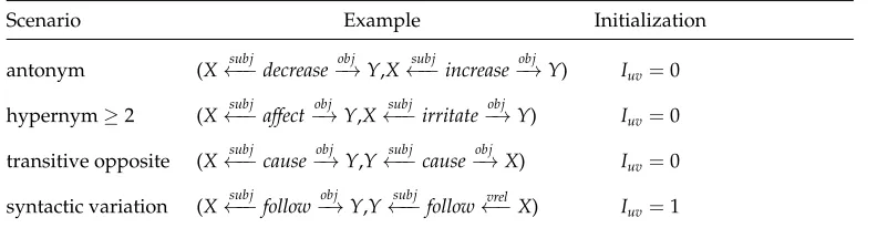
As mentioned in Section 4.2, we added a few constraints in cases where there was strong evidence that edges are not in the graph. This is done in the following scenarios (examples given in Table 3): (1) When two templatesu andv are identical except for a pair of words w_u and w_v, and w_u is an antonym of w_v, or a hypernym of w_v at distance≥2 in WordNet. (2) When two nodesuandvare transitive “opposites,” that is, ifu=X←−−subj w−→obj Yandv=X←−obj w−−→subj Y, for any wordw. We note that there are some transitive verbs that express a reciprocal activity, such asX marries Y, but usually reciprocal events are not expressed using a transitive verb structure.

In addition, in some cases we have strong evidence that edges do exist in the graph. This is done in a single scenario (see Table 3), which is specific to the output of Minipar: when two templates differ by a single edge and the first is of the type X−→obj Yand the other is of the typeX←−−vrel Y, which expresses a passive verb modifier of nouns. Altogether, these initializations took place in less than 1% of the node pairs in the graphs. We note that we tried to use WordNet relations such as hypernym and synonym as “positive” hard constraints (using the constraintIuv=1), but this resulted in reduced performance because the precision of WordNet was not high enough.

The graphs learned by our algorithm were evaluated by two measures. The first measure evaluates the graph edges directly, and the second measure is motivated by semantic inference applications that utilize the rules in the graph. The first measure is simply theF₁ of the set of learned edges compared to the set of gold-standard edges. In the second measure we take the set of learned rules and infer new propositions by applying the rules over all propositions extracted from the health-care corpus. We apply the rules iteratively over all propositions until no new propositions are inferred. For example, given the corpus propositionrelaxation reduces nauseaand the edgesX reduces nausea→ X helps with nausea and X helps with nausea→ X related to nausea, we eval-uate the set{relaxation reduces nausea, relaxation helps with nausea, relaxation related to nausea}. For each graph we measure theF1 of the set of propositions inferred by the

learned graphs when compared to the set of propositions inferred by the gold-standard graphs. For both measures the final score of an algorithm is a macro-averageF1 over

the 24 gold-standard test-set graphs (two gold-standard graphs for each of the 12 test concepts).

Table 3

Scenarios in which we added hard constraints to the ILP.

Scenario Example Initialization

antonym (X←−−subj decrease−→obj Y,X←−−subj increase−→obj Y) Iuv=0

hypernym≥2 (X←−−subj affect−→obj Y,X←−−subj irritate−→obj Y) Iuv=0

transitive opposite (X←−−subj cause−→obj Y,Y←−−subj cause−→obj X) Iuv=0

Learning the edges of a graph given an input concept takes about 1–2 seconds on a standard desktop.

5.2 Evaluated Algorithms

First, we describe some baselines that do not utilize the entailment classifier or the ILP solver. For each of the 16 distributional similarity measures (Table 2) and for each templatet, we computed a list of templates most similar tot(or entailingtfor directional measures). Then, for each measure we learned graphs by inserting an edge (u,v), when uis in the topKtemplates most similar tov. The parameterKcan be optimized either on the automatically generated training set (from WordNet) or on the manually annotated development set. We also learned graphs using WordNet: We inserted an edge (u,v) whenuandvdiffer by a single wordwuandwv, respectively, andwuis a direct hyponym or synonym ofwv. Next, we describe algorithms that utilize the entailment classifier.

Our algorithm, namedILP-Global, utilizes global information and an ILP formula-tion to find maximum a posteriori graphs. Therefore, we compare it to the following three variants: (1) ILP-Local: An algorithm that uses only local information. This is done by omitting the global transitivity constraints, and results in an algorithm that inserts an edge (u,v) if and only if (Suv−λ)>0. (2)Greedy-Global: An algorithm that looks for the maximum a posteriori graphs but only employs the greedy optimization procedure as described by Snow, Jurafsky, and Ng (2006). (3)ILP-Global-Likelihood: An ILP formulation where we look for the maximum likelihood graphs, as described by Snow, Jurafsky, and Ng (cf. Section 4.2).

We evaluate these algorithms in three settings which differ in the method by which the edge prior odds ratio, η(orλ), is estimated: (1)η=1 (λ=0), which means that no prior is used. (2) Tuningηand using the value that maximizes performance over the development set. (3) Estimatingηusing maximum likelihood over the development set, which results inη∼0.1 (λ∼2.3), corresponding to the edge densityP(Iuv=1)∼0.09.

For all local algorithms whose output does not respect transitivity constraints, we added all edges inferred by transitivity. This was done because we assume that the rules learned are to be used in the context of an inference or entailment system. Because such systems usually perform chaining of entailment rules (Raina, Ng, and Manning 2005; Bar-Haim et al. 2007; Harmeling 2009), we conduct this chaining as well. Nevertheless, we also measured performance when edges inferred by transitivity are not added: We once again chose the edge prior value that maximizes F1 over the development set

and obtained macro-average recall/precision/F1of 51.5/34.9/38.3. This performance is

comparable to the macro-average recall/precision/F1of 44.5/45.3/38.1 we report next

in Table 4.

5.3 Experimental Results and Analysis

In this section we present experimental results and analysis that show that the ILP-Global algorithm improves performance over baselines, specifically in terms of precision.

Tables 4–7 and Figure 2 summarize the performance of the algorithms. Table 4 shows our main result when the parametersλ andKare optimized to maximize per-formance over the development set. Notice that the algorithm ILP-Global-Likelihood is omitted, because when optimizing λ over the development set it conflates with ILP-Global. The rowsLocal1 and Local2 present the best algorithms that use a single

Table 4

Results when tuning for performance over the development set.

Edges Propositions

Recall Precision F1 Recall Precision F1

ILP-Global (λ=0.45) 46.0 50.1 43.8 67.3 69.6 66.2

Greedy-Global (λ=0.3) 45.7 37.1 36.6 64.2 57.2 56.3 ILP-Local (λ=1.5) 44.5 45.3 38.1 65.2 61.0 58.6 Local1(K=10) 53.5 34.9 37.5 73.5 50.6 56.1 Local2(K=55) 52.5 31.6 37.7 69.8 50.0 57.1

Table 5

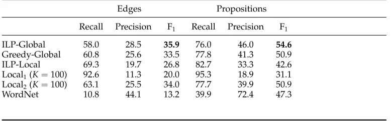
Results when the development set is not used to estimateλandK.

Edges Propositions

Recall Precision F1 Recall Precision F1

ILP-Global 58.0 28.5 35.9 76.0 46.0 54.6

Greedy-Global 60.8 25.6 33.5 77.8 41.3 50.9 ILP-Local 69.3 19.7 26.8 82.7 33.3 42.6 Local1(K=100) 92.6 11.3 20.0 95.3 18.9 31.1 Local2(K=100) 63.1 25.5 34.0 77.7 39.9 50.9 WordNet 10.8 44.1 13.2 39.9 72.4 47.3

Table 6

Results with prior estimated on the development set, that isη=0.1, which is equivalent to λ=2.3.

Edges Propositions

Recall Precision F1 Recall Precision F1

ILP-Global 16.8 67.1 24.4 43.9 86.8 56.3

ILP-Global-Likelihood 91.8 9.8 17.5 94.0 16.7 28.0 Greedy-Global 14.7 62.9 21.2 43.5 86.6 56.2 Greedy-Global-Likelihood 100.0 9.3 16.8 100.0 15.5 26.5

described in Table 2 by features no. 5 and no. 1, respectively (see also Table 8). ILP-Global improves performance by at least 13%, and significantly outperforms all local methods, as well as the greedy optimization algorithm both on the edges F1 measure

(p<0.05) and on the propositions F1measure (p<0.01).10

Table 5 describes the results when the development set is not used to estimate the parameters λ and K: A uniform prior (Puv=0.5) is assumed for algorithms that use the entailment classifier, and the automatically generated training set is employed to estimateK. Again ILP-Global-Likelihood is omitted in the absence of a prior. ILP-Global outperforms all other methods in this scenario as well, although by a smaller margin for a few of the baselines. Comparing Table 4 to Table 5 reveals that excluding the

Table 7

Results per concept for the ILP-Global.

Concept R P F1

Smoking 58.1 81.8 67.9 Seizure 64.7 51.2 57.1 Headache 60.9 50.0 54.9 Lungs 50.0 56.5 53.1 Diarrhea 42.1 60.0 49.5 Chemotherapy 44.7 52.5 48.3 HPV 35.2 76.0 48.1 Salmonella 27.3 80.0 40.7 X-ray 75.0 23.1 35.3 Asthma 23.1 30.6 26.3 Mouth 17.7 35.5 23.7 FDA 53.3 15.1 23.5

sparse prior indeed increases recall at a price of a sharp decrease in precision. Note, however, that local algorithms are more vulnerable to this phenomenon. This makes sense because in local algorithms eliminating the prior adds edges that in turn add more edges due to the constraint of transitivity and so recall dramatically rises at the expense of precision. Global algorithms are not as prone to this effect because they refrain from adding edges that eventually lead to the addition of many unwarranted edges.

Table 5 also shows that WordNet, a manually constructed resource, has notably the highest precision and lowest recall. The low recall exemplifies how the entailment relations given by the gold-standard annotators transcend much beyond simple lexical relations that appear in WordNet: Many of the gold-standard entailment relations are missing from WordNet or involve multi-word phrases that do not appear in WordNet at all.

Note that although the precision of WordNet is the highest in Table 5, its absolute value (44.1%) is far from perfect. This illustrates that hierarchies of predicates are quite

Figure 2

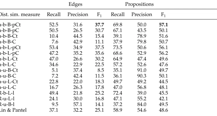
Table 8

Results of all distributional similarity measures when tuningKover the development set. We encode the description of the measures presented in Table 2 in the following manner— h = health-care corpus;R = RCV1 corpus;b = binary templates;u = unary templates;L = Lin similarity measure;B = BInc similarity measure;pCt = pair of CUI tuples representation;pC = pair of CUIs representation;Ct = CUI tuple representation;C = CUI representation;Lin & Pantel = similarity lists learned by Lin and Pantel.

Edges Propositions

Dist. sim. measure Recall Precision F1 Recall Precision F1

h-b-B-pCt 52.5 31.6 37.7 69.8 50.0 57.1

h-b-B-pC 50.5 26.5 30.7 67.1 43.5 50.1 h-b-B-Ct 10.4 44.5 15.4 39.1 78.9 51.6 h-b-B-C 7.6 42.9 11.1 37.9 79.8 50.7 h-b-L-pCt 53.4 34.9 37.5 73.5 50.6 56.1 h-b-L-pC 47.2 35.2 35.6 68.6 52.9 56.2 h-b-L-Ct 47.0 26.6 30.2 64.9 47.4 49.6 h-b-L-C 34.6 22.9 22.5 57.2 52.6 47.6 h-u-B-Ct 5.1 37.4 8.5 35.1 91.0 49.7 h-u-B-C 7.2 42.4 11.5 36.1 90.3 50.1 h-u-L-Ct 22.8 22.0 18.3 49.7 49.2 44.5 h-u-L-C 16.7 26.3 17.8 47.0 56.8 48.1 R-b-L-l 49.4 21.8 25.2 72.4 39.0 45.5 R-u-L-l 24.1 30.0 16.8 47.1 55.2 42.1 R-u-B-l 9.5 57.1 14.1 37.2 84.0 49.5 Lin & Pantel 37.1 32.2 25.1 58.9 54.6 48.6

ambiguous and thus using WordNet directly yields relatively low precision. WordNet is vulnerable to such ambiguity because it is a generic domain-independent resource, whereas our algorithm learns from a domain-specific corpus. For example, the words have and cause are synonyms according to one of the senses in WordNet and so the erroneous rule X have asthma ↔ X cause asthma is learned using WordNet. Another example is the ruleX follows chemotherapy→X takes chemotherapy, which is incorrectly inferred becausefollowis a hyponym oftakeaccording to one of WordNet’s senses (she followed the feminist movement). Due to these mistakes made by WordNet, the precision achieved by our automatically trained ILP-Global algorithm when tuning parameters on the development set (Table 4) is higher than that of WordNet.

a purely probabilistic approach that will allow us to reach good performance when estimating η directly. Nevertheless, currently optimal results are achieved when the priorηis tuned empirically.

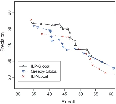
Figure 2 shows a recall–precision curve for Global, Greedy-Global, and ILP-Local, obtained by varying the prior parameter,λ. The figure clearly demonstrates the advantage of using global information and ILP. ILP-Global is better than Greedy-Global and ILP-Local in almost every point of the recall–precision curve, regardless of the exact value of the prior parameter. Last, we present for completeness in Table 7 the results of ILP-Global for all concepts in the test set.

In Table 8 we present the results obtained for all 16 distributional similarity mea-sures. The main conclusion we can derive from this table is that the best distributional similarity measures are those that represent templates using pairsof argument instan-tiations rather than each argument separately. A similar result was found by Yates and Etzioni (2009), who described the RESOLVER paraphrase learning system and have shown that it outperforms DIRT. In their analysis, they attribute this result to their representation that utilizes pairs of arguments comparing to DIRT, which computes a separate score for each argument.

In the next two sections we perform a more thorough qualitative and quantitative comparison trying to analyze the importance of using global information in graph learning (Section 5.3.1), as well as the contribution of using ILP rather than a greedy optimization procedure (Section 5.3.2). We note that the analysis presented in both sec-tions is for the results obtained when optimizing parameters over the development set.

5.3.1 Global vs. Local Information. We looked at all edges in the test-set graphs where ILP-Global and ILP-Local disagree and checked which algorithm was correct. Table 9 presents the result. The main advantage of using ILP-Global is that it avoids inserting wrong edges into the graph. This is because ILP-Local adds any edge (u,v) such that Puvcrosses a certain threshold, disregarding edges that will be consequently added due to transitivity (recall that for local algorithms we add edges inferred by transitivity, cf. Section 5.2). ILP-Global will avoid such edges of high probability if it results in inserting many low probability edges. This results in an improvement in precision, as exhibited by Table 4.

Figures 3 and 4 show fragments of the graphs learned by Global and ILP-Local (prior to adding transitive edges) for the test-set concepts diarrheaand seizure, and illustrate qualitatively how global considerations improve precision. In Figure 3, we witness that the single erroneous edge X results in diarrhea → X prevents diarrhea inserted by the local algorithm because P_uv is high, effectively bridges two strongly connected components and induces a total of 12 wrong edges (all edges from the upper component to the lower component), whereas ILP-Global refrains from inserting this edge. Figure 4 depicts an even more complex scenario. First, ILP-Local induces a strongly connected component of five nodes for the predicates control, treat, stop,

Table 9

Comparing disagreements between ILP-Global and ILP-Local against the gold-standard graphs.

Global=True/Local=False Global=False/Local=True

Gold standard=true 48 42

Figure 3

A comparison between ILP-Global and ILP-local for two fragments of the test-set concept diarrhea.

reduce, andprevent, whereas ILP-Global splits this strongly connected component into two, which although not perfect, is more compatible with the gold-standard graphs. In addition, ILP-Local inserts four erroneous edges that connect two components of size 4 and 5, which results in adding eventually 30 wrong edges. On the other hand,

Figure 4

ILP-Global is aware of the consequences of adding these four seemingly good edges, and prefers to omit them from the learned graph, leading to much higher precision.

Although the main contribution of ILP-Global, in terms of F1, is in an increase in

precision, we also notice an increase in recall in Table 4. This is because the optimal prior isλ=0.45 in ILP-Global butλ=1.5 in ILP-Local. Thus, any edge (u,v) such that 0.45<Suv<1.5 will have positive weight in ILP-Global and might be inserted into the graph, but will have negative weight in ILP-Local and will be rejected. The reason is that in a local setting, reducing false positives is handled only by applying a large penalty for every wrong edge, whereas in a global setting wrong edges can be rejected because they induce more “bad” edges. Overall, this leads to an improved recall in ILP-Global. This also explains why ILP-Local is severely harmed when no prior is used at all, as shown in Table 5.

Last, we note that across the 12 test-set graphs, ILP-Global achieves betterF1 over

the edges in 7 graphs with an average advantage of 11.7 points, ILP-Local achieves betterF1over the edges in 4 graphs with an average advantage of 3.0 points, and one

performance is equal.

5.3.2 Greedy vs. Non-Greedy Optimization. We would like to understand how using an ILP solver improves performance compared with a greedy optimization procedure. Table 4 demonstrates that ILP-Global and Greedy-Global reach a similar level of re-call, although ILP-Global achieves far better precision. Again, we investigated edges for which the two algorithms disagree and checked which one was correct. Table 10 demonstrates that the higher precision is because ILP-Global avoids inserting wrong edges into the graph.

Figure 5 illustrates some of the reasons ILP-Global performs better than Greedy-Global. Parts A1–A3 show the progression of Greedy-Global, which is an incremental algorithm, for a fragment of theheadachegraph. In part A1 the learning algorithm still separates the nodesX prevents headacheandX reduces headachefrom the nodesX causes headache and X results in headache(nodes surrounded by a bold oval shape constitute a strongly connected component). After two iterations, however, the four nodes are joined into a single strongly connected component, which is an error in principle but at this point seems to be the best decision to increase the posterior probability of the graph. This greedy decision has two negative ramifications. First, the strongly connected component can no longer be untied. Thus, in A3 we observe that in future iterations the strongly connected component expands further and many more wrong edges are inserted into the graph. On the other hand, in B we see that ILP-Global takes into consideration the global interaction between the four nodes and other nodes of the graph, and decides to split this strongly connected component in two, which improves the precision of ILP-Global. Second, note that in A3 the nodesAssociate X with headache andAssociate headache with Xare erroneously isolated. This is because connecting them to the strongly connected component that contains six nodes will add many edges with

Table 10

Comparing disagreements between ILP-Global and Greedy-Global against the gold-standard graphs.

ILP=True/Greedy=False ILP=False/Greedy=True

Gold standard=true 66 56

Figure 5

A comparison between ILP-Global and Greedy-Global. Parts A1–A3 depict the incremental progress of Greedy Global for a fragment of theheadachegraph. Part B depicts the corresponding fragment in ILP-Global. Nodes surrounded by a bold oval shape are strongly connected

components.

low probability and so this is avoided by Greedy-Global. Because in ILP-Global the strongly connected component was split in two, it is possible to connect these two nodes to some of the other nodes and raise the recall of ILP-Global. Thus, we see that greedy optimization might get stuck in local maxima and consequently suffer in terms of both precision and recall.

Last, we note that across the 12 test-set graphs, ILP-Global achieves betterF1 over

the edges in 9 graphs with an average advantage of 10.0 points, Greedy-Global achieves betterF₁over the edges in 2 graphs with an average advantage of 1.5 points, and in one case performance is equal.

5.4 Error Analysis