Estimation of Location (μ) and Scale (λ) for Two Parameter Half Logistic Pareto Distribution (HLPD) by Least Square Regression Method

(1)

Estimation of Location (μ) and Scale (λ) for Two

-Parameter Half Logistic Pareto Distribution

(HLPD) by Least Square Regression Method

M. Vijayalakshmi1, G. V. S. R. Anjaneyulu2

1

Research Scholar (BSRRFSMS), 2Professor, Department of Statistics,Acharya Nagarjuna University, Guntur, Andhra Pradesh, India.

Abstract: In this paper, we propose the estimation of Location (µ) and Scale (λ) parameters using two step least square estimation method. We also computed Average Estimate (AE), Variance (VAR), Standard Deviation (STD), Mean Absolute Deviation (MAD), Mean Square Error (MSE), Simulated Error (SE) and Relative Absolute Bias (RAB) for both the parameters under complete sample based on 1000 simulations to assess the performance of the estimators. In this paper, finally we shows that the best performance of Least Square Regression Estimation Method.

Keywords: Two parameter HLP distribution, median ranks method (Benard's approximation), Least Square method, Montecarlo Simulation.

I. INTRODUCTION

Generally in many of the sciences, we face some type of situations of non monotonic failure rates for supervise the reliability analysis of the data under carefully scrutinize. In order to model such data, Aarset, M. V. (1987). Swain, J., Venkataraman, S. & Wilson, J. R. (1988) proposed Least squares estimatimators and Weighted Least squares estimators of a Beta distribution. For an excellent review for the two distributions the readers are referred to Johnson, Kotz and Balakrishnan (1995) .Madholkaretal (1995) present an extension of the Weibull family that not only contains unimodel distribution with bath tub failure rates but also allows for a broader class of monotone hazards rates and is computationally convenient for censored data. They named their extended version as “Exponentiated Weibull Family”. On similar lines Gupta and Kundu (2001b) proposed a new model called generalized exponential distribution. A generalized (type – II) version of logistic distribution was considered and some interesting properties of the distribution were derived by Balakrishnan and Hassain (2007). Ramakrishna (2008) studied the Type I generalized half logistic

distribution scale (σ) and shape (θ) parameters estimation using the least square method in two step estimation methods. Torabi and Bagheri (2010) consider different parameter estimation methods in extended generalized half logistic distribution for censored as well as complete sample. Rama Mohan, ch. and Anjaneyulu, G. V. S. R. (2011) studied how the least square method be good for estimating the parameters to Two Parameter Weibull Distribution from an optimally constructed grouped sample. Kantam et al (2013) discussed the estimation and testing in Type I generalized half logistic distribution. Rama Mohan, CH and Anjaneyulu, GVSR (2014) was studied estimation of scale and shape parameters of type I generalized half logistic distribution using Median Ranks Method. In section - 1.2, we discussed the procedure to estimate of Scale (



) and Shape (



) parameters of HLPD by

using the Least Square Regression Method. Hence it term these estimators as Least Squares method.

In section – 1.3 we presented observations and conclusions are based on simulation results with numerical example.

If Let X1, X2,..., Xn be a random sample of size n from HLPD

( , )

 

is a probability model, its probability density function (pdf),

cumulative distribution function (cdf) and Hazard Function (HF) are given by

f(x) = f(x: β,



) =

1

2 2 x x

 







  

 

, x



0 ... (1.1.1)

F(x) = F(x:

 

, )

= x x

 

 

 

, x



0

... (1.1.2) H(x) = H(

x

; ,

 

) = x 1

x



 

 

 

(2)

II. ESTIMATION OF SCALE (



) AND SHAPE (



) PARAMETERS OF TWO PARAMETER

A. HLPD using Least Square Regression Method

Let x1< x2< x3………..< xN be an ordered sample of size ‘N’ from Half Logistic Pareto Distribution with the parameters Scale (



)

and Shape (



). Then the cdf is

given as in equation (1.1.2), can be written as

2

1

F x

( )

x



 









_{... (1.2.1)}

and

2

1

F x

( )

x

  









_{... (1.2.2)}

1

( )

1

( )

F x

x

 









... (1.2.3) Taking Logarithm on both side of equation (1.2.3), we get

1

( )

log

1

( )

F x

x

F x



























_{... (1.2.4)}

From the least square parameter estimation method (also known as regression analysis), we have,

A= log ,

exp(

),

,

1

( )

log

,

log

1

( )

A

B

and

F x

U

V

x

F x



 





 























... (1.2.5) 2

1 1 1 1

2 2

1 1

n n n n

i i i i i

i i i i

n n

i i

v

u

v

v u

A

n

v

     



 





 







 





 





 





 







 







 





 







... (1.2.6)

1 1 1

2 2

1 1

n n n

i i i i

i i i

n n

i i

n v u v u

B

n v v

                                     



 ... (1.2.7)

B. Simulation Study

In order to obtain the median ranks method estimators of Scale (



) and Shape (



) are obtained and study the properties of their

estimates through the Average Estimate (AE), Variance (VAR), Mean Square Error (MSE) and Relative Absolute Bias (RAB) and Relative Error under in order to obtain the Median Ranks Method estimators of Scale (



) and Shape (



)and study the properties

complete sample are given respectively by forgiven values of n,



and



. If is Median Ranks Method estimate of , m=1,

(3)

Average Estimate ( ) =∑

Variance ( ) = ∑ ( )

Mean Absolute Deviation = ∑ ( )

Mean Square Error ( ) = ∑ ( )

Relative Absolute Bias ( ) =∑ ( )

Relative Error( ) =

∑ ( )

III. OBSERVATIONS FROM SIMULATION RESULTS AND CONCLUSIONS.

1) The Average Estimate (AE), Variance (VAR), Standard deviation ( STD), Mean Square Error (MSE) and Relative Absolute Bias (RAB) are independent of true values of the parameters of of scale (



) and Shape (



) .

2) Average Estimate (AE) of scale parameter (





) were increasing when sample size (N) is increasing.

3) Variance (VAR) of scale parameter (





) and shape parameter (





) by Least Square Method were decreasing when sample

size (N) is increasing.

4) Standard Deviation (STD) of scale parameter (









) by Least Square Method were decreasing

when sample size (N) is increasing.

5) Mean Absolute Deviation (MAD) of scale (









) by Least Squares Method were decreasing

6) Mean Square Error (MSE) of scale parameter (









7) Simulated Error(SE) in Average Estimate (AE), Variance (VAR), Standard Deviation (STD), Mean Square Error (MSE) and

Relative Absolute Bias (RAB) of scale parameter (









8) Relative Absolute Bias (RAB) of scale parameter (





)) and shape parameter (





9) Scale parameter (





) by Least Square Method is having less variance(VAR).

10) Scale parameter (









) by Least Square Method having less Standard deviation.

A. Numerical Example

We generate a random sample of size 10 with scale (



) = 0.5 and shape (



) = 3 of HLPD and the order sample is given by 0.37,

2.46, 2.89, 3.28, 3.59, 3.98, 4.56, 5.47, 8.25, 9.23. Solving equations (3.3.6) and (3.3.7) for this simple data and the resulting estimators of the scale (



) and shape (



) of HLPD as follows:

Scale Parameter Medians Rank method



ˆ

= 0.25672 Shape Parameter Medians Rank method



ˆ

= 2.3.4567

(4)

1) Simulated Data: The Average Estimate(AE), Variance(VAR), Mean Square Error(MSE) and Relative Absolute Bias(RAB), Relative Error(RE) of Least Square method estimators of scale and shape parameters under complete sample of 1000 simulations. Population parameters Scale=0.5 and Shape = 3 in Table-1.1.

Table 1.1

Sample size

Para meters

Average

Estimation Variance MAD MSE RAB RE

50 0.145892 0.00427 0.08371 0.12539 0.35411 0.17705

1.271366 0.30723 0.690501 2.98818 0.28811 0.86432

100 0.144203 0.00306 0.079635 0.12659 0.71159 0.1779

1.479711 0.60649 0.921707 2.31128 0.50676 0.76014

150 0.190193 0.01079 0.128935 0.09598 0.1549 0.1549

0.980956 0.29872 0.721972 4.07654 1.00952 1.00952

200 0.241152 0.02022 0.186359 0.067 1.03539 0.12942

1.44426 0.37095 0.818894 2.42033 1.03716 0.77787

250 0.252815 0.0163 0.168259 0.0611 1.23593 0.12359

1.509687 0.36595 0.765655 2.22103 1.24193 0.74516

300 0.247445 0.0169 0.178204 0.06378 1.51533 0.12628

2.529393 0.32663 0.757875 0.22147 0.47061 0.2353

350 0.258414 0.01538 0.155983 0.05836 1.6911 0.12079

2.508062 0.26704 0.646877 0.242 0.57393 0.24597

400 0.317106 0.02112 0.17595 0.03345 1.46315 0.09145

2.486837 0.23908 0.600144 0.26334 0.68422 0.25658

450 0.295101 0.02371 0.191071 0.04198 1.84409 0.10245

2.446952 0.21625 0.626062 0.30586 0.82957 0.27652

500 0.301234 0.02071 0.184539 0.03951 1.98766 0.09938

2.757186 0.02158 0.194464 0.05896 0.40469 0.12141

ˆ

ˆ ˆ

2) Simulated Data: The Average Estimate(AE), Variance(VAR), Mean Square Error(MSE) and Relative Absolute Bias(RAB), Relative Error(RE) of Least Square method estimators of scale and shape parameters under complete sample of 1000 simulations. Population parameters Scale=1.5 and Shape =2 in Table-1.2.

Table 1.2

n

Para meters

Average

Estimation Variance MAD MSE RAB RE

50 0.8236966 0.452514 0.21839 0.457386 0.323697 0.004509 1.217976 0.571732 0.67458 0.611562 0.195506 0.00391 100 0.9431828 0.231694 0.2841 0.310045 0.886366 0.003712 1.257106 0.556472 0.5357 0.551892 0.371447 0.003714 150 1.0495562 0.220089 0.3744 0.2029 0.274778 0.003003 1.428822 0.436436 0.72573 0.326244 0.428383 0.003138 200 0.957831 0.21332 0.56579 0.293947 0.831324 0.003614 1.372304 0.412985 0.60652 0.394002 0.627696 0.002977 250 1.0695903 0.20432 0.54866 0.149178 0.068822 0.002575 1.538986 0.352885 0.75995 0.212534 0.576267 0.002856 300 1.1137644 0.19558 0.59524 0.185252 0.417542 0.002869 1.40451 0.315787 0.68634 0.354608 0.893235 0.002305 350 1.2247195 0.190634 0.5875 0.075779 0.073037 0.001835 1.659454 0.300334 0.92333 0.115972 0.595956 0.001703 400 1.2355012 0.086303 0.5883 0.06996 0.88401 0.001763 1.722293 0.272567 0.80607 0.077121 0.471498 0.001389 450 1.2588825 0.051789 0.57599 0.058138 0.829943 0.001607

ˆ

ˆ



ˆ

(5)

[image:5.612.78.534.134.394.2]

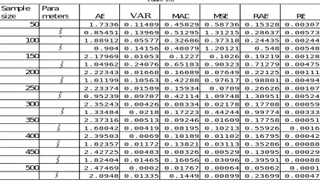
The Average Estimate(AE), Variance(VAR), Mean Square Error(MSE) and Relative Absolute Bias(RAB), Relative Error(RE) of Least Square method estimators of scale and shape parameters under complete sample of 1000 simulations. Population parameters Scale=2.5 and Shape = 2 in Table-1.3.

Table-1.3

Sample size

Para

meters AE VAR MAD MSE RAB RE

50 1.7336 0.11489 0.45829 0.58736 0.15328 0.00307

0.85451 0.13969 0.51295 1.31215 0.28637 0.00573

100 1.88912 0.05577 0.32686 0.37318 0.24435 0.00244

0.904 0.14156 0.48079 1.20121 0.548 0.00548

150 2.17969 0.01053 0.1227 0.1026 0.19219 0.00128

1.04962 0.24076 0.65183 0.90323 0.71279 0.00475

200 2.22343 0.01668 0.16089 0.07649 0.22125 0.00111

1.01199 0.10563 0.42288 0.97617 0.98801 0.00494

250 2.23374 0.01589 0.15934 0.0709 0.26626 0.00107

0.95239 0.09707 0.42114 1.09748 1.30951 0.00524

300 2.35243 0.00426 0.08334 0.02178 0.17708 0.00059

1.33484 0.0218 0.17223 0.44244 0.99774 0.00333

350 2.37316 0.00513 0.09246 0.01609 0.17758 0.00051

1.68042 0.00419 0.08195 0.10213 0.55926 0.0016

400 2.39503 0.0069 0.10189 0.01102 0.16795 0.00042

1.82357 0.01172 0.13821 0.03113 0.35286 0.00088

450 2.42725 0.00483 0.08326 0.00529 0.13095 0.00029

1.82404 0.01465 0.16056 0.03096 0.39591 0.00088

500 2.47469 0.0002 0.01767 0.00064 0.05062 0.0001

2.0948 0.01335 0.1449 0.00899 0.23699 0.00047

ˆ

ˆ ˆ

ˆ

ˆ ˆ

Table 1.4

Sample size

Para

50 2.76281 0.14946 0.52337 0.069069 0.05256 0.00105

1.83449 0.15445 0.47002 0.027394 0.04138 0.00083

100 2.85768 0.0431 0.24859 0.127936 0.14307 0.00143

1.84271 0.14594 0.47134 0.024742 0.07865 0.00079

150 3.1891 0.01096 0.1087 0.474859 0.41346 0.00276

2.12153 0.22421 0.59686 0.014770 0.09115 0.00061

200 2.80416 0.1675 0.50875 0.092513 0.24333 0.00122

2.00114 0.10585 0.3828 0.000001 0.00114 0.00001

250 3.24995 0.01443 0.14298 0.562417 0.74994 0.003

1.97314 0.09224 0.36713 0.000722 0.03358 0.00013

300 3.34328 0.00431 0.07446 0.711122 1.01194 0.00337

2.31846 0.02524 0.20054 0.101416 0.47769 0.00159

350 3.36409 0.00492 0.08878 0.746656 1.20973 0.00346

2.68707 0.00466 0.08804 0.472065 1.20237 0.00344

400 3.3905 0.00809 0.11715 0.792998 1.42481 0.00356

2.66799 0.00038 0.02627 0.446213 1.33598 0.00334

450 3.42326 0.005 0.08841 0.852409 1.66187 0.00369

2.81983 0.014 0.15231 0.672127 1.84463 0.00410

500 3.47603 0.0002 0.01827 0.952639 1.95206 0.0039

3.11576 0.01306 0.14073 1.244909 2.78939 0.00558

ˆ

(6)

Table 1.5

Sample size

Para

50 0.17192 0.00541 0.07389 0.10874 0.32975 0.0066

0.57075 0.06398 0.2779 0.27151 0.26053 0.00521

100 0.14683 0.00278 0.0729 0.13393 0.73192 0.00732

0.50665 0.1012 0.33759 0.21322 0.46176 0.00462

150 0.23062 0.00525 0.07564 0.06695 0.77621 0.00517

0.65201 0.07125 0.31304 0.11426 0.50704 0.00338

200 0.25646 0.01843 0.17941 0.06429 1.01425 0.00507

0.76824 0.02982 0.23072 0.06586 0.51326 0.00257

250 0.25389 0.01744 0.15848 0.06363 1.26126 0.00505

0.7504 0.02946 0.2193 0.05908 0.60767 0.00243

300 0.23866 0.01512 0.17289 0.06667 1.5492 0.00516

0.80965 0.02005 0.17354 0.03564 0.56633 0.00189

350 0.30794 0.01079 0.13196 0.03606 1.32927 0.0038

0.81477 0.01983 0.19523 0.03211 0.62715 0.00179

400 0.39312 0.00816 0.11427 0.01176 0.86751 0.00217

0.85889 0.01916 0.16564 0.01684 0.51913 0.0013

450 0.42085 0.00564 0.10043 0.00575 0.68223 0.00152

0.82569 0.01336 0.14943 0.03397 0.82943 0.00184

500 0.47442 0.00022 0.0176 0.00059 0.24363 0.00049

0.96475 0.0014 0.04654 0.00111 0.16621 0.00033

ˆ

ˆ ˆ

ˆ

ˆ ˆ

The Average Estimate (AE), Variance(VAR), Mean Square Error(MSE) and Relative Absolute Bias(RAB), Relative Error(RE) of Least Square method estimators of scale and shape parameters under complete sample of 1000 simulations. Population parameters Scale=1.5 and Shape = 3 in Table-1.6.

Table 1.6 Sample

size

Para

50 1.17531 0.00489 0.09012 0.10542 0.10823 0.00216

2.44372 0.09077 0.2976 0.30944 0.09271 0.00185

100 1.14391 0.0027 0.05959 0.1268 0.23739 0.00237

2.49467 0.09937 0.42249 0.25536 0.16844 0.00168

150 1.24251 0.0056 0.09259 0.0663 0.25749 0.00172

2.63544 0.05812 0.29203 0.1329 0.18228 0.00122

200 1.25176 0.01729 0.1632 0.06162 0.33098 0.00165

2.72722 0.03004 0.23285 0.07441 0.18185 0.00091

250 1.23038 0.01657 0.1576 0.07269 0.44936 0.0018

2.75367 0.0288 0.22873 0.06068 0.20527 0.00082

300 1.2426 0.01811 0.17798 0.06626 0.5148 0.00172

2.82288 0.02015 0.19377 0.03137 0.17712 0.00059

350 1.30292 0.00996 0.12808 0.03884 0.45986 0.00131

2.81254 0.02507 0.21484 0.03514 0.2187 0.00062

400 1.40003 0.00788 0.11261 0.00999 0.26658 0.00067

2.86893 0.0168 0.16351 0.01718 0.17476 0.00044

450 1.42764 0.00489 0.08811 0.00524 0.21709 0.00048

2.82585 0.01385 0.15351 0.03033 0.26122 0.00058

500 1.47515 0.00021 0.01787 0.00062 0.08282 0.00017

ˆ

(7)

REFERENCES

[1] Aarset, M.V. (1987). How to identify a bathtub shaped hazard rate? IEEE Transactions on Reliability, 36, 106 – 108

[2] Abd-Elfattah, A. M., Hassan, A. S. & Ziedan, D. M. (2006). Efficiency of maximum likelihood estimators under different censored sampling schemes for Rayleigh distribution. Interstat, March issue, 1.

[3] Dey, S. (2009). Comparison of Bayes Estimators of the parameter and reliability function for Rayleigh distribution under different loss functions. Malaysian Journal of Mathematical Sciences, 3, 247 - 264.

[4] Dey, S. & Das, M.K. (2007). A Note on Prediction Interval for a Rayleigh Distribution: Bayesian Approach. American Journal of Mathematical and Management Science, 1&2, 43 - 48.

[5] Johnson, N.L., Kotz, S. and Balakrishnan, N. (1995), Continuous Univariate Distribution Vol. 1, 2nd Ed., New York, Wiley.

[6] Khan, H.M.R., Provost, S.B. & Singh, A. (2010). Predictive inference from a two-parameter Rayleigh life model given a doubly censored sample. Communications in Statistics - Theory and Methods, 39, 1237 - 1246.

[7] Kantam, R.R.L, Ramakrishna, V. and Ravikumar, M.S. (2013). Estimation and testing in type 1 generalized half logistic distribution. Modern applied statistical methods, Vol. 12, No. 1, PP. 198-206.

[8] Kundu, D. & Raqab, M.Z. (2005). Generalized Rayleigh distribution: different methods of estimation. Computational Statistics and Data Analysis, 49, 187 - 200.

[9] Rayleigh, J.W.S. (1880). On the resultant of a large number of vibrations of the Some pitch and of arbitrary phase. Philosophical Magazine, 5-th Series, 10, 73 - 78.

[10] Rama Mohan, ch. And Anjaneyulu, G. V. S, R. : How the Least Square Method be good for Estimating the parameters to Two-Parameter Weibull distribution from an optimally constructed grouped sample. International Journal of Statistics and Systems, (2011) Vol. 6,pp. 525-535.

[11] Ramamohan, C. H., Anjaneyulu, G. V. S. R. and Suresh Kumar, P. (2014). Estimation of Scale parameter (σ) when Shape parameter (β) is known in Log

Logistic Distribution using Minimum Spaceing Square Distance Estimation Method from an optimally constructed grouped sample. ICRASTAT2013 conference proceedings, Department of Statistics, Dr. Babasaheb Ambedkar Marathwada University, Aurangabad. (Accepted for publication)

[12] Swain, J., Venkataraman, S. & Wilson, J.R. (1988). Least squares estimation of distribution functions in Johnson’s translation system. Journal of Statistical Computation and Simulation, 29, 271 - 297.

[13] Torabi, H., Bagheri, F.L. :Estimation of Parameters for an Extended Generalized Half Logistic Distribution Based on completed and Censored Data. JIRSS(2010), Vol.9, No.2, pp. 171-195.