Control objective : In this paper, an adaptive decoupled

Abstract—In this paper, we propose a novel SPSA-based on-line adaptive decoupled control scheme by using PID neural network for a class of nonlinear systems. In addition, the update laws of parameters with adaptive optimal learning rate are proposed based on the Lyapunov stability theorem, this guarantees the stability of closed-loop system. In addition, the affect of the frictional force model and uncertainty are discussed and analyzes. The proposed approach is applied in the translational oscillations with a rotational actuator (TORA) system. In experimental results, the proposed control is realized by DSP to demonstrate the performance and the efficiency.

Index Terms—adaptive control, PID neural network, simultaneous perturbation stochastic approximation, real-time control.

I. INTRODUCTION

ECENTLY, intelligent control systems using fuzzy logic system and neural networks are widely applied for particular systems [2, 11-12, 14, 17]. The neural networks are used to approximate the complicated mathematical function of nonlinear systems when the physical mathematical model is not exactly known. For the training of neural networks, there are many optimization problems which only the measurement of the objective function is available. To develop the neural-network-based controller, the corresponding adaptive laws should be derived by the measurement of objective function. Many approaches were introduced to train the neural networks [5, 9, 11-12, 14-15, 17-18]. However, the usually used methods are gradient descent method and Lyapunov approach. However, it is difficult to obtain the system’s gradient information exactly. Therefore, the simultaneous perturbation stochastic approximation (SPSA) is proposed to solve these problems [23, 27-29]. By using SPSA, we can only measure the objective function to solve the optimization problem for providing the adaptive laws of neural networks.

In this paper, we propose a novel SPSA-based on-line adaptive decoupled control scheme by using PID neural network for a class of nonlinear systems. The sliding-mode

This work was supported in part by the National Science Council, Taiwan, R.O.C., under contracts NSC-97-2221-E-155-033-MY3.

Ching-Hung Lee is with Department of Electrical Engineering, Yuan-Ze University, Chung-li, Taoyuan 320, Taiwan. (phone: +886-3-4638800, ext: 7119; fax: +886-3-4639355, e-mail: chlee@saturn.yzu.edu.tw).

control (SMC) has been suggested as an approach for the control of systems with nonlinearities, uncertain dynamics and bounded input disturbances [1-2, 7-10, 21, 22, 24]. The SMC-based decoupled architecture is adopted for simplifying the computational complexity. The weights of the PID NN are updated according to the results of SPSA algorithm for the purpose of controlling the system states to stay in sliding surface. By using the SPSA update laws, we can adjust the PID neural network’s parameters to achieve the stability of closed-loop system. The proposed approach is applied in the translational oscillations with a rotational actuator (TORA) system. In experimental results, the proposed control is realized by DSP to demonstrate the performance and the efficiency.

This paper is organized as follows. Section II introduces the problem formulations and PID neural networks. The proposed on-line adaptive decoupled control scheme is introduced in Section III. Experimental results of TORA system are shown in Section IV. Finally, the conclusion is given.

II. PRELIMINARIES A. Problem Formulation

Consider the following nonlinear coupled system

( )

1

( )

1, 1

1 13 12

12 11

d u g f x

x x

x x

n = + ⋅ +

= =

X X

& M & &

( )

2

( )

2, 2

2 23 22

22 21

d u g f x

x x

x x

n = + ⋅ +

= =

X X

& M & &

y1=x1,y2=x2 (1)

where T T T _{x x x}n _{x x x}n1 T 2n

21 21 21 1 11 11 11 2

1 ] [ ... ... ]

[ = ∈ℜ

= − −

& &

X X

X is

system state variable and y1,y2∈ℜ are system output.

( ) ( )

X, i X ∈ℜ,

i g

f i=1,2, which satisfy gi

( )

X ≠0, ∀X≠0, .

0

≥

t u is the control input, and d1(t), d2(t), are external

bounded disturbances, i.e., |d1(t)|≤D1, |d2(t)|≤D2.

Control objective: In this paper, an adaptive decoupled PID neural network controller is proposed to treat the tracking control problem of system (1), that is the proposed controller generates proper control signal such that the system output y1 and y2 follows the continuous bounded

desired trajectories yr1 and yr2, respectively. Note that the

desired trajectories yr1, yr2∈Cn-1, i.e., the (n-1)th order

derivative exist. Thus, we define

Adaptive Neural Network Controller Design

for a Class of Nonlinear Systems Using SPSA

Algorithm

Ching-Hung Lee, Member, IAENG, Tsung-Min Yu, and Jen-Chieh Chien

T n r r

r T n r r

r r

T n r r

r T n r r

r r

x x

x x

x x

x x

x x

x x

] [

] [

] [

] [

2 22

21 )

1 (

21 21

21 2

1 12

11 )

1 (

11 11

11 1

L L

&

L L

&

= =

= =

− − X

X

(2) and the error states are defined as

2 2 2

1 1 1

ri ri

X X e

X X e

− =

− =

. (3) Therefore, our control objective is transfer into generating proper control signals such that e1 and e2 converge to zero

when t→∞.

) (k kD

) (k k_I

) (k kP

∑

1

− z

)

(

k

e

)

2

(

)

1

(

2

)

(

k

−

e

k

−

+

e

k

−

e

)

1

(

)

(

k

−

e

k

−

e

) (k u )

(k kD

) (k k_I

) (k kP

∑

∑

1

− z−1

z

)

(

k

e

)

2

(

)

1

(

2

)

(

k

−

e

k

−

+

e

k

−

e

)

1

(

)

(

k

−

e

k

−

e

[image:2.595.58.283.185.277.2]

) (k u

Fig. 1. The structure of PID neural network.

B. PID Neural Network

The proportional integral derivative (PID) controllers are still widely used in process industries even though control theory has been developed significantly since they were first used decades ago. Most of industrial controllers are still implemented based around PID algorithms, particularly at lowest levels, robustness, applicability, and ease of use offered by the PID controller [19]. In addition, neural networks have been applied in many areas including nonlinear control, classification, intelligent control, signal processing, image processing, etc [5, 9-12, 14-15, 17, 19-20, 24, 30-31, 32-33]. Herein, we adopt PID NN controller with adaptive learning rates to produce the control signals. The structure of PID neural network is shown in Fig. 1, the corresponding control input is

)] 1 ( ) ( )[ ( ) ( ) (

)] 2 ( ) 1 ( 2 ) ( )[ ( ) 1 ( ) (

− − +

+

− + − − +

− =

k e k e k k k e k k

k e k e k e k k k u k u

P I

D

(4) where kp(k), kI(k), kD(k) are adaptive adjustable parameters.

In our previous literature [16], the gradient-descent method was adopted to derive the adaptive update laws for kp(k), kI(k),

and kD(k). However, the system uncertainty, external

disturbance, internal noise, and frictional force are unknown. This implies the worse performance of control problem. For solving the problem, we propose an adaptive decoupled PID neural network controller using the SPSA algorithm and SMC technique.

C. Simultaneous Perturbation Stochastic Approximation (SPSA) Algorithm

This section introduces the SPSA algorithm briefly. The detail description can be found in literature [16]. Consider a problem of finding the minimum of objective function f(W). The SPSA algorithm computes the parameter W at next iteration as

)) ( ( ) ( ) ( ) 1

(k W k ak gW k

W + = − (5) where (.)g is estimated gradient result for objective function f(.), i.e., ( ) g(W)

W W

f _≈

∂ ∂

. a(k) is the learning step length

which is decreased over iterations with

₍

₎

α

A k a k

a( )= ₊ ,

where a, A, and α are positive configuration coefficients [16]. The SPSA approach estimates the gradient g(.) using following method. Assume that the dimension of parameter W is p. Let Δ(k)=

[

Δ1(k) Δ2(k) ... Δp(k)

]

be a

p-dimensional vector whose element is mutually independent zero-mean random variable. Then, the estimation of the gradient at kth iteration can be computed by SPSA algorithm

) (

)) ( ( )) ( ) ( ) ( ( )) ( (

k c

k W f k k c k W f k W

g = + Δ −

[

]

T

p(k) ... (k)

(k) 1 1

2 1 1

− −

− _{Δ Δ}

Δ

⋅ (6) where c(k)= c_(k+1)γ is gain sequence, where c and γ are nonnegative configuration coefficients. Obviously, all the elements of the parameter W are perturbed simultaneously, and only two measurement of the objective function are needed to estimate the gradient. In addition, Δ(k) is usually obtained using Bernoulli ±1 distribution with equal probability for each value.

[image:2.595.307.549.409.525.2]

In general, the gradient information of neural fuzzy system is not easy to obtain due to the asymmetric membership functions and interval valued sets. Herein, we adopt the SPSA algorithm to derive the stable learning rule which guarantees the convergence and stability of the closed-loop systems.

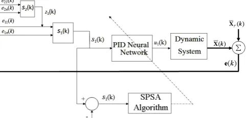
Fig. 3. The proposed decoupled PIDNN control scheme

III. DESIGN OF DECOUPLED CONTROLLER USING SPSA ALGORITHM

A. SMC- based Decoupled Control Design

According equation (3), we define the corresponding sliding mode surface as

1 11 1 1

1 c z

s _=cT_{e − and}

2 2

2 c e

T

s = (7) where ( )

1 2 1 1

Φ

=z sat s

z U is called the decoupled factor [22].

sat(.) denotes the saturation function

⎩ ⎨ ⎧

< ≥ =

1 | | ,

1 | | ), sgn( ) (

x if x

x if x x

sat (8)

Herein, c1=[c11 c12 … c1n-1]T and c2=[c21 c22 L c2n−1 1]Tare

chosen properly such that all eigenvalues of s1=0, s2 =0

the PID neural network based decoupled adaptive control scheme using SPSA algorithm. The inputs of PID neural network are s1 and the output is the control signal for

nonlinear system.

Our control goal is to minimize the following cost function: ) ( 2 1 ) ( 2 1 k s k

E = . (9) By the gradient-descent method, the update laws of ith PIDNN’s parameters are

⎥ ⎥ ⎥ ⎥ ⎥ ⎥ ⎥ ⎦ ⎤ ⎢ ⎢ ⎢ ⎢ ⎢ ⎢ ⎢ ⎣ ⎡ ∂ ∂∂ ∂ ∂ ∂ ⎥ ⎥ ⎥ ⎦ ⎤ ⎢ ⎢ ⎢ ⎣ ⎡ − ⎥ ⎥ ⎥ ⎦ ⎤ ⎢ ⎢ ⎢ ⎣ ⎡ = ⎥ ⎥ ⎥ ⎦ ⎤ ⎢ ⎢ ⎢ ⎣ ⎡ + + + D I p D I P D I p D I p k k Ek k E k k E k a k a k a k k k k k k k k k k k k ) ( ) ( ) ( ) ( 0 0 0 ) ( 0 0 0 ) ( ) ( ) ( ) ( ) 1 ( ) 1 ( ) 1 ( (10)

where aP(k),aI(k), aD(k) are adaptive time varying learning

step length. Herein, we use the SPSA algorithm to approximate the gradients of

p k k E ∂ ∂ ( ) _, I k k E ∂ ∂ ( )_, D k k E ∂

∂ ( )_{, thus}

⎥ ⎥ ⎥ ⎥ ⎥ ⎥ ⎥ ⎦ ⎤ ⎢ ⎢ ⎢ ⎢ ⎢ ⎢ ⎢ ⎣ ⎡ Δ ⋅ −Δ ⋅ − Δ ⋅ − = ⎥ ⎥ ⎥ ⎥ ⎥ ⎥ ⎥ ⎦ ⎤ ⎢ ⎢ ⎢ ⎢ ⎢ ⎢ ⎢ ⎣ ⎡ Δ ⋅ + −

+ ⋅Δ

+ − + Δ ⋅ + − + ≈ ⎥ ⎥ ⎥ ⎥ ⎥ ⎥ ⎥ ⎦ ⎤ ⎢ ⎢ ⎢ ⎢ ⎢ ⎢ ⎢ ⎣ ⎡ ∂ ∂∂ ∂ ∂ ∂ Δ Δ Δ Δ Δ Δ Δ Δ Δ Δ Δ Δ ) ( ) ( )) ( ( )) ( ( ) ( ) ( )) ( ( )) ( ( ) ( ) ( )) ( ( )) ( ( ) ( ) ( ) 1 ( ) 1 ( ) ( ) ( ) 1 ( ) 1 ( ) ( ) ( ) 1 ( ) 1 ( ) ( ) ( ) ( k k c k E k E k k c k E k E k k c k E k E k k c k E k E k k c k E k E k k c k E k E k k E k k E k k E D I p D I p D I p W W W W W W (11)

where T

D I

p k k k k k

k

k) [ ( ) ( ) ( )]

( =

W , WΔ(k)=[kp(k)

) ( ) ( )

(k k k k

c ⋅Δp I

+ Δ +cΔ(k)⋅ΔI(k) kD(k)+cΔ(k)

T ] ) (k D Δ ⋅

,cΔ(k)∈ℜ is perturbation that between 0 and 1. ΔP(k), )

(k I

Δ , ΔD(k) are perturbation ones whose elements are

either 1 or -1 in random.

From equations (10) and (11), the update laws of kp(k),

kI(k), kD(k) are represented as

) ( ) ( ) ( ) ( ) ( ) ( ) ( ) ( ) ( ) ( ))] ( ( [ ) ( ) ( ) ( ) 1 ( 1 1 1 1 k k c k s k k c k k c k s k k c k g k s k a k k k k p D p I P P P Δ ⋅ Δ ⋅ + ⎢ ⎢ ⎣ ⎡ Δ ⋅ ⋅ Δ ⋅ ⋅ ⋅ ⋅ − = + Δ Δ Δ Δ X ) ( ) ( )] 2 ( ) 1 ( 2 )[ ( )

( 1 1

k k c k s k s k k c p D Δ ⋅ − + − − Δ ⋅ + Δ Δ ⎥ ⎦ ⎤ Δ ⋅ − − Δ ⋅ + Δ Δ ) ( ) ( )] 1 ( ) ( )[ ( )

( 1 1

k k c k s k s k k c P

P ₍₁₂₎

) ( ) ( ) ( ) ( ) ( ) ( ) ( ) ( ) ( ) ( ))] ( ( [ ) ( ) ( ) ( ) 1 ( 1 1 1 1 k k c k s k k c k k c k s k k c k g k s k a k k k k I D I I I I I Δ ⋅ Δ ⋅ + ⎢ ⎣ ⎡ Δ ⋅ ⋅ Δ ⋅ ⋅ ⋅ ⋅ − = + Δ Δ Δ Δ X ) ( ) ( )] 2 ( ) 1 ( 2 )[ ( )

( _{1 1}

k k c k s k s k k c I D Δ ⋅ − + − − Δ ⋅ + Δ Δ ⎥ ⎦ ⎤ Δ ⋅ − − Δ ⋅ + Δ Δ ) ( ) ( )] 1 ( ) ( )[ ( )

( 1 1

k k c k s k s k k c I

P ₍₁₃₎

) ( ) ( ) ( ) ( ) ( ) ( ) ( ) ( ) ( ) ( ))] ( ( [ ) ( ) ( ) ( ) 1 ( 1 1 1 1 k k c k s k k c k k c k s k k c k g k s k a k k k k D D D I D D D Δ ⋅ Δ ⋅ + ⎢ ⎣ ⎡ Δ ⋅ ⋅ Δ ⋅ ⋅ ⋅ ⋅ − = + Δ Δ Δ Δ X ) ( ) ( )] 2 ( ) 1 ( 2 )[ ( )

( 1 1

k k c k s k s k k c D D Δ ⋅ − + − − Δ ⋅ + Δ Δ ⎥ ⎦ ⎤ Δ ⋅ − − Δ ⋅ + Δ Δ ) ( ) ( )] 1 ( ) ( )[ ( )

( 1 1

k k c k s k s k k c D

P _{. (14)}

B. Stability analysis

Herein, we develop the convergence theorem for selecting appropriate learning step length a(k). The choice of learning step length is very important for convergence. If a small value is given for the learning step length, the convergence of the closed-loop system is guaranteed. However, the convergent speed may be very slow. On the other hand, if a large value is given, the system may be unstable. Hence, we employ the Lyapunov stability analysis approach to have the condition for convergence and find the optimal learning step length. We have the following theorem for control scheme.

Theorem 1. Let aP(k), aI(k), aD(k) be adaptive learning

step length for PID neural network tuning parameters. Consider the nonlinear control problem (shown in Fig. 3), the asymptotic convergence of the closed-loop system is guarantee if the learning step length is chosen satisfying

2 ) ( 2 ) ( 0 k g k a <

< , for all k (15) where ) ( )) ( ( )) ( ) ( ) ( ( )) (

( 1 1

k c k W s k k c k W s k W

g = + Δ −

[

]

T

p(k) ... (k)

(k) 1 1

2 1 1

− −

− _{Δ Δ}

Δ ⋅

is the gradient estimation using SPSA approach. In addition, the faster convergence can be obtained by using the following optimal time-varying learning step length

(

( )- ( -1)

) (

( )

)

] ) 3[ 1 , 1 min( ) ( ₂ 1 1

1 k s k g k

s k aP X =

(

( )

)

] ) ) ( 3[ 1 , 1 min( ) ( 2 1

1 k g k

s k

aI

X

= (16)

(

( )-2 ( -1) ( -2)

) (

( )

)

] ) 3[ 1 , 1 min( ) ( 2 1 1 1

1 k s k s k g k

s k aD X + =

Proof: The proof is omitted due to the writing space.

[image:4.595.58.276.56.145.2]

Fig. 5. Experimental equipment of the developed TORA systems at YZU.

IV. APPLICATION IN NONLINEAR TORASYSTEM AND EXPERIMENTAL RESULTS

In the early 1990s, Bupp et. al proposed a benchmark problem for nonlinear control design [3-4, 26]. This benchmark problem consists of the motion control of a cart possessing one translational degree of freedom, which is actuated by an eccentric rotational mass actuator mounted on the cart. The system of cart and rotational actuator is referred to as the so-called TORA system or RTAC (Rotational/Translational Actuator) system. The schematic representation of the TORA system is shown in Fig. 4, which comprises a cart of mass M that is connected to a spring of stiffness K fixed to a wall. The cart is perturbed by a disturbance force F. There is a rotating arm of mass m and length e in the center of the cart. The pendulum is actuated by the control input N. The cart and pendulum move in the horizontal plane, where xc and x&c denote the normalized

translational position and velocity of the cart, respectively, and θ and θ& denote the angular position and velocity of the rotational actuator [13].

Based on the generalized coordinates _{[x ,x , , ]}T C

C & θ θ& , the

motion equations of an ideal TORA system are

. cos )

(

) sin cos

( )

( 2

2

N

θ

x me

θ

me I

F me

Kx x m M

c c c

+ −

= +

+ −

− = + +

&& &&

& &&

&& θ θ θ θ

(17) The torque N is generated by the DC motor and is proportional to the current i fed to the motor, i.e., N=kTi,

where kT=18.26 mN/A is the motor constant. By the

following normalization and state transformation, we have the following state space representation

( ) ( )

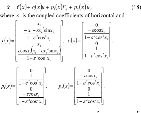
x g xu p

( )

xFd p

( )

x ud f

x&= + + 1 + 2 (18)

where ε is the coupled coefficients of horizontal and

( )

(

)

,

cos 1

sin cos

cos 1

sin

3 2 2

3 2 4 1 3

4 3 2 2

3 2 4 1

2

⎥ ⎥ ⎥ ⎥ ⎥ ⎥ ⎥

⎦ ⎤

⎢ ⎢ ⎢ ⎢ ⎢ ⎢ ⎢

⎣ ⎡

− − −

+ −

=

x x x x x

x x

x x x

x

x f

ε ε ε

ε ε

( )

,

cos 1

1 0 cos 1

cos0

3 2 2

3 2 2

3

⎥ ⎥ ⎥ ⎥ ⎥ ⎥

⎦ ⎤

⎢ ⎢ ⎢ ⎢ ⎢ ⎢

⎣ ⎡

− − − =

x x x

x g

ε ε ε

( )

,

cos 1

cos0 cos 1

1 0

3 2 2

3 3 2 2

1

⎥ ⎥ ⎥ ⎥ ⎥ ⎥

⎦ ⎤

⎢ ⎢ ⎢ ⎢ ⎢ ⎢

⎣ ⎡

− − − =

x x

x x

p

ε ε

ε

_{( )}

.

cos 1

1 0 cos 1

cos0

3 2 2

3 2 2

3

2

⎥ ⎥ ⎥ ⎥ ⎥ ⎥

⎦ ⎤

⎢ ⎢ ⎢ ⎢ ⎢ ⎢

⎣ ⎡

− − − =

x x x

x p

ε ε ε

According system (1), we define

[

]

T x x x

x111, 112, 121, 122 =

x

=

[

]

T

d

d x

x ,_& ,θ,θ& . The experimental setup consists of a DC

motor, a motor driver, a personal computer, a D/A control card, an open-type linear scale, and a rotational encoder and is located in the Intelligent Control and Applications Laboratory at Yuan Ze University. The experimental equipment of developed TORA system is shown in Fig. 5.

Case1: Stability Illustration (system having frictional force)

In this simulation, coefficients are chosen as zU11 =0.9, 10

11=

φ , c111=10, c121=0.5. The TORA initial condition is T

x=[0.07000] . PIDNN initial parameters are set to be kP=0, kI=0, kD=0 and the friction force are identified as [13]

( )

c c

f x x

F =1.33& +0.5sgn & , Nf =0.01θ&+0.04sgn

( )

θ&. (19)

0 1 2 3 4 5 6 7 8 9 10

-0.5 0 0.5

time(sec)

θ

System Response

0 1 2 3 4 5 6 7 8 9 10

-0.05 0 0.05 0.1 0.15

time(sec)

xc

System Response

desired output adaptive PID-BP DNNSMC Our approach desired output adaptive PID-BP DNNSMC Our approach

Fig. 6. Comparison results (dotted: PID-BP [16]; dashed: DNN SMC [6]; solid: our approach).

0 2 4 6 8 10

-20 0 20 40

time(sec)

u

(a) Control Effort

0 0.2 0.4 0.6 0.8 1

-10 0 10 20 30 40

time(sec)

u

(b) Control Effort Time:0~1sec

adaptive PID-BP DNNSMC Our approach

[image:4.595.305.540.171.741.2]

adaptive PID-BP DNNSMC Our approach

Fig. 7. Comparison results of control effort (dotted: PID-BP [16]; dashed: DNN SMC [6]; solid: our approach).

0 1 2 3 4 5 6 7 8 9 10 -0.5

0 0.5 1

time(sec)

θ

0 1 2 3 4 5 6 7 8 9 10 -5

0 5

time(sec)

u

0 1 2 3 4 5 6 7 8 9 10 -0.1

0 0.1

time(sec)

xc

η=1.2

η=0.01 Our approach desired output

η=1.2

η=0.01 Our approach desired output

η=1.2

η=0.01 Our approach

Fig. 8. Comparison results using difference learning step lengths (dashed: fixed value 1.2; dotted: fixed value: 0.01; solid: our approach in equation

[image:4.595.47.290.558.753.2]

Figure 6 shows the simulation results when the system having frictional force. We can observe that the proposed approach has the better performance in convergence. The corresponding control effort is shown in Fig. 7. Figure 7(b) shows the control effort between 0~1 sec. It is also found that the proposed approach has more reasonable control effort than other literature [6, 16]. Figure 8 shows the simulation results of our approach using difference fixed learning step length and adaptive step length (16). Also, we find that the proposed adaptive learning step length performs well by using SPSA.

0 1 2 3 4 5 6 7 8 9 10

-0.15 -0.1 -0.05 0 0.05 0.1 0.15

time(sec)

θ

System Response

0 1 2 3 4 5 6 7 8 9 10

-0.01 -0.005 0 0.005 0.01

time(sec)

xc

System Response

desired output adaptive PID-BP DNNSMC Our approach adaptive PID-BP DNNSMC Our approach

Fig. 9. Comparison results of oscillation control (dotted: PID-BP [16]; dashed: DNN SMC [6]; solid: our approach).

0 1 2 3 4 5 6 7 8 9 10

-10 -5 0 5

time(sec)

u

Control Effort

0 0.2 0.4 0.6 0.8 1 1.2 1.4 1.6 1.8 2 -10

-5 0 5 10

time(sec)

u

Control Effort

[image:5.595.333.508.167.292.2] [image:5.595.64.273.201.558.2]

adaptive PID-BP DNNSMC Our approach adaptive PID-BP DNNSMC Our approach

Fig. 10. Comparison results in control effort of oscillation control (dotted: PID-BP [16]; dashed: DNN SMC [6]; solid: our approach).

Case2: Oscillation Control Illustration (system having frictional force)

In addition, we use the following illustrated examples, oscillation control problem, to show that the controller can reduce the influence of uncertainty. These are used to demonstrate the effectiveness and ability of the proposed control scheme. The initial conditions of the following oscillation control are selected as xC

( )

0 =0 [m],

( )

0 =0 C

x& [m/s], θ(0)=0[deg] and θ&

( )

0 =0[deg/s], and the desired trajectory is derived from the oscillation frequency, i.e., xcd =0.005sin(10.15t). The Oscillation control case is

considered.

As above, Fig. 9 shows the simulation results when the system having frictional force. We can observe that the proposed approach has the better performance in

[image:5.595.80.260.221.365.2]

convergence. The corresponding control effort is shown in Fig. 10, Fig. 10(b) is control effort between 0 to 1 sec. It is also found that the proposed approach has more reasonable control effort than other literature [6, 16]. Figure 11 shows the simulation results of our approach using difference fixed learning step length and adaptive step length (16). Also, we find that the proposed adaptive learning step length performs well by using SPSA.

0 1 2 3 4 5 6 7 8 9 10 -0.5

0 0.5

time(sec)

θ

0 1 2 3 4 5 6 7 8 9 10 -0.02

0 0.02 0.04

time(sec)

xc

desired output

η=1.2

η=0.01 Our approach

0 1 2 3 4 5 6 7 8 9 10 -10

0 10

time(sec)

u

desired

η=1.2

η=0.01 Our approach

η=1.2

η=0.01 Our approach

Fig. 11. Comparison results of oscillation control case using difference learning step lengths (dashed: fixed value 1.2; dotted: fixed value: 0.01; solid:

[image:5.595.328.528.339.455.2]

our approach in equation (16)).

Fig. 12. DSP-based control platform for the TORA system.

Experimental Results of TORA System using DSP-based Control Scheme

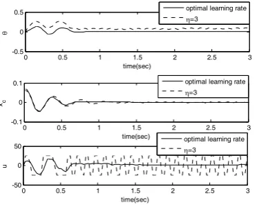
The experimental equipment block diagram of the DSP-based control system f or the TORA system are depicted in Fig. 12. Figure 13 shows the experimental result of stability problem. The proposed approach has good performance (converge to zero in small stabilizing time) in experimental equipment. Figure 14 shows the state trajectories of our approach with fixed learning step length and adaptive step length (16). This result illustrates the effectiveness and ability of the adaptive learning step length.

0 0.5 1 1.5 2 2.5 3

-0.1 0 0.1

time(sec)

xc

0 0.5 1 1.5 2 2.5 3

-50 0 50

time(sec)

u

0 0.5 1 1.5 2 2.5 3

-0.2 0 0.2

time(sec)

[image:5.595.332.515.629.768.2]

θ

0 0.5 1 1.5 2 2.5 3 -0.5

0 0.5

time(sec)

θ

0 0.5 1 1.5 2 2.5 3

-50 0 50

time(sec)

u

optimal learning rate

η=3

0 0.5 1 1.5 2 2.5 3

-0.1 0 0.1

time(sec)

xc

optimal learning rate

η=3

optimal learning rate

[image:6.595.74.262.57.207.2]

η=3

Fig. 14. Comparison results of experimental results by using fixed learning step length and adaptive step length (16).

V. CONCLUSION

In this paper, we have proposed a novel SPSA-based on-line adaptive decoupled control scheme by using PID neural network for a class of nonlinear systems. In addition, the update laws of parameters with adaptive optimal learning rate are proposed based on the Lyapunov stability theorem, this guarantees the stability and performance of closed-loop system. The affect of the frictional force model and uncertainty are discussed and analyzes. The proposed approach is applied in the TORA system. In experimental results, the proposed control has been realized by DSP to demonstrate the performance and the efficiency.

REFERENCES

[1] G. Bartolini, E. Punta, and T. Zolezzi, “Simplex methods for nonlinear uncertain sliding-mode control,” IEEE Trans. on

Automatic Control, Vol. 49, No. 6, pp. 922–933, 2004.

[2] G. D. Buckner, “Intelligent bounds on modeling uncertainty: Applications to sliding-mode control,” IEEE Trans. on Sys., Man and

Cyb., Part C,Vol. 32, No. 2, pp. 113–124, 2002.

[3] R. T. Bupp, D. S. Bernstein, and V. T. Coppola, “A benchmark problem for nonlinear control design: Problem statement, experimental testbed, and passive nonlinear compensation,” Proc.

American Control Conf., pp. 4363–4367, 1995.

[4] R. T. Bupp, et al., “Special Issue: a nonlinear benchmark problem,”

Int. J. of Robust Nonlinear Control, Edited by D. S. Bernstein, Vol. 8,

No.4, pp. 305-457, John Wiley Sons, 1998.

[5] D. E. Goldberg, Genetic Algorithms in Search, Optimization and

Machine Learning, Addison-Wesley, Reading, 1989.

[6] L. C. Hung and H. Y. Chung, “Decoupled control using neural network-based sliding-mode controller for nonlinear systems,”

Expert Systems with Application, Vol. 32, No. 4, pp. 1168-1182,

2007.

[7] L. C. Hung and H. Y. Chung , “Decoupled sliding-mode with fuzzy-neural network controller for nonlinear systems,” Expert

Systems with Application, Vol. 46, No. 1, pp. 74-97, 2007.

[8] M. A. Hussain and P. Y. Ho, “Adaptive sliding-mode control with neural network based hybrid models,” J. of Proc. Control, Vol. 14, No. 2, pp. 157–176, 2004.

[9] J. Kennedy and R. Eberhart, “Particle swarm optimization,” IEEE Int.

Conf. Neural Networks, Perth, Australia, pp. 1942-1948, 1995.

[10] M. Krstic, J. Sun, and P. V. Kokotovic, “Robust control of nonlinear systems with input unmodeled dynamics,” IEEE Trans. on Automatic.

Control, Vol. 41, No. 6, pp. 913-920, 1996.

[11] C. H. Lee and C. C. Teng, “Identification and control of dynamic systems using recurrent fuzzy neural networks,” IEEE Trans. on

Fuzzy Sys., Vol. 8, No. 4, pp. 349-366, 2000.

[12] C. H. Lee, P. C. Kuo, M. A. Kuo, and M. H. Chiu, “A hybrid learning algorithm for fuzzy neural network using GA and BP,” The 10th

Fuzzy Theory and Its Applications Conf., Hsinchu, Taiwan, 2002.

[13] C. H. Lee and S. K. Chang, “Experimental Implementation of

Nonlinear TORA System and Robust Adaptive Backstepping Controller Design,” Accepted to appear in Neural Computing and

Applications, Dec. 2010.

[14] C. H. Lee, “Stabilization of nonlinear nonminimum phase systems: an adaptive parallel approach using recurrent fuzzy neural network,”

IEEE Trans. on Sys., Man, Cyb.- Part: B, Vol. 34, No. 2, pp.

1075-1088, 2004.

[15] C. H. Lee and Y. C. Lin, “Hybrid learning algorithm for fuzzy neural systems,” IEEE Int. Conf. on Fuzzy Sys., Vol. 2, pp. 691-696, 2004. [16] C. H. Lee and C. C. Teng, “Control of a nonlinear dynamic system via

adaptive PID control scheme with saturation bound,” International

Journal of Fuzzy Sys., Vol. 4, No. 4, pp. 922-927, 2002.

[17] C. H. Lee and J. C. Chien, “Fuzzy-neural-based decoupled controller design of nonlinear multi-input-multi-output system,” The 17th

National Conf. on Fuzzy Theory and Its Applications, pp. 213-218,

2009.

[18] C. H. Lee, C. T. Kuo, and H. H. Chang, “Preformance enhancement of differential evoluation algorithm using local search and self-adaptive scaling factor,” CACS Int. Automatic Control Conf., pp. 850-855, 2009.

[19] C. J. Lin, C. Y. Lee, and C. C. Chin, “Dynamic recurrent wavelet network controllers for nonlinear system control,” J. of The Chinese

Institute of Engineers, Vol. 29, No. 4, pp. 747-751, 2006.

[20] C. J. Lin and Y. C. Hsu, “Reinforcement hybrid evolutionary learning for recurrent wavelet-based neuro-fuzzy systems,” IEEE Trans. on

Fuzzy Sys., Vol. 15, No. 4, pp. 729-745, 2007.

[21] C. M. Lin and Y. J. Mon, “Decoupling control by hierarchical fuzzy sliding-mode controller,” IEEE Trans. on Control Sys. Technology, Vol. 13, No. 4, pp. 593-598, 2005.

[22] J. C. Lo and Y. H. Kuo, “Decoupled fuzzy sliding-mode control,”

IEEE Trans. on Fuzzy Sys., Vol. 6, No. 3, pp. 426–435, 1998.

[23] Y. Maeda, “Simultaneous perturbation learning rule for recurrent neural networks and Its FPGA implementation,” IEEE Trans. on

Neural Networks, Vol. 16, No. 6, pp. 1664-1672, 2005.

[24] M. Onder Efe, O. Kayanak, X. Yu, and B. Wilamowski, “ Sliding Mode Control of Nonlinear Systems Using Gaussian Radial Basis Function Neural Networks,” Proc. of the IJCNN, Washington D.C., USA, pp. 474-479, 15-19 July 2001.

[25] R. Ordónez and K. M. Passino, “Stable multi-input multi-output adaptive fuzzy/neural control,” IEEE Trans. on Fuzzy Sys., Vol. 7, No. 3, pp. 345-353, 1999.

[26] A. Pavlov, B. Janssen, N. van de Wouw, and H. Nijmeijer, “Experimental output regulation for a nonlinear benchmark system,”

IEEE Trans. on Control Systems Technology, Vol. 15, pp. 786-793,

2007.

[27] J. C. Spall, “Multivariate stochastic approximation using a simultaneous perturbation gradient approximation,” IEEE Trans. on

Automatic Control, Vol. 37, No. 3, pp. 332–341, 1992.

[28] J. C. Spall, “Implementation of the simultaneous perturbation algorithm for stochastic optimization,” IEEE Trans. on Aerospace

and Electronic Sys., Vol. 34, No. 3, 1998.

[29] J. C. Spall, “An overview of the simultaneous perturbation method for efficient optimization,” Johns Hopkins APL Technical Digest, Vol. 19, No. 4, 1998.

[30] F. Sun and H. X. Li, “Neuro-fuzzy dynamic-inversion-based adaptive control for robotic manipulators-discrete time case,” IEEE Trans. on

Ind. Electronics,Vol. 54, No. 3, pp. 1342-1351, 2007.

[31] J. S. Wang and Y. P. Chen, “A fully automated recurrent neural network for unknown dynamic system identification and control,”

IEEE Trans. on Cir. and Sys.-I, Vol. 56, No. 6, pp. 1363-1372, 2006.

[32] S. Zhou, G. Feng, and C. B. Feng, “Robust control for a class of uncertain nonlinear systems: adaptive fuzzy approach based on backstepping,” Fuzzy Sets and Sys., Vol. 151, No. 1, pp. 1-20, 2005. [33] J. Zilkova, J. Timko, and P. Girovsky, “Nonlinear system control