Compression of Neural Machine Translation Models via Pruning

Compression of Neural Machine Translation Models via Pruning

Abigail See∗ _{Minh-Thang Luong}∗ _{Christopher D. Manning}

Computer Science Department, Stanford University, Stanford, CA 94305

{abisee,lmthang,manning}@stanford.edu

Abstract

Neural Machine Translation (NMT), like many other deep learning domains, typ-ically suffers from over-parameterization, resulting in large storage sizes. This paper examines three simple magnitude-based pruning schemes to compress NMT mod-els, namely class-blind, class-uniform, and class-distribution, which differ in terms of how pruning thresholds are com-puted for the different classes of weights in the NMT architecture. We demonstrate the efficacy of weight pruning as a compres-sion technique for a state-of-the-art NMT system. We show that an NMT model with over 200 million parameters can be pruned by 40% with very little performance loss as measured on the WMT’14 English-German translation task. This sheds light on the distribution of redundancy in the NMT architecture. Our main result is that withretraining, we can recover and even surpass the original performance with an 80%-pruned model.

1 Introduction

Neural Machine Translation (NMT) is a simple new architecture for translating texts from one lan-guage into another (Sutskever et al., 2014; Cho et al., 2014). NMT is a single deep neural network that is trained end-to-end, holding several advan-tages such as the ability to capture long-range de-pendencies in sentences, and generalization to un-seen texts. Despite being relatively new, NMT has already achieved state-of-the-art translation re-sults for several language pairs including English-French (Luong et al., 2015b), English-German (Jean et al., 2015a; Luong et al., 2015a; Luong and

∗_{Both authors contributed equally.}

student   a   am  

I   Je  

Je   suis  

suis   étudiant     étudiant     _  

_  

source  language  input   target  language  input   target  language  output  

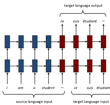
Figure 1: A simplified diagram of NMT.

Manning, 2015; Sennrich et al., 2016), English-Turkish (Sennrich et al., 2016), and English-Czech (Jean et al., 2015b; Luong and Manning, 2016). Figure 1 gives an example of an NMT system.

While NMT has a significantly smaller memory footprint than traditional phrase-based approaches (which need to store gigantic phrase-tables and language models), the model size of NMT is still prohibitively large for mobile devices. For exam-ple, a recent state-of-the-art NMT system requires over 200 million parameters, resulting in a stor-age size of hundreds of megabytes (Luong et al., 2015a). Though the trend for bigger and deeper neural networks has brought great progress, it has also introduced over-parameterization, resulting in long running times, overfitting, and the storage size issue discussed above. A solution to the over-parameterization problem could potentially aid all three issues, though the first (long running times) is outside the scope of this paper.

Our contribution. In this paper we investi-gate the efficacy of weight pruning for NMT as a means of compression. We show that despite

its simplicity, magnitude-based pruning with re-training is highly effective, and we compare three magnitude-based pruning schemes —class-blind,

class-uniform andclass-distribution. Though re-cent work has chosen to use the latter two, we find the first and simplest scheme — class-blind

— the most successful. We are able to prune 40% of the weights of a state-of-the-art NMT system with negligible performance loss, and by adding a retraining phase after pruning, we can prune 80% with no performance loss. Our pruning experi-ments also reveal some patterns in the distribution of redundancy in NMT. In particular we find that higher layers, attention and softmax weights are the most important, while lower layers and the em-bedding weights hold a lot of redundancy. For the Long Short-Term Memory (LSTM) architecture, we find that at lower layers the parameters for the input are most crucial, but at higher layers the pa-rameters for the gates also become important.

2 Related Work

Pruning the parameters from a neural network, referred to as weight pruning or network prun-ing, is a well-established idea though it can be implemented in many ways. Among the most popular are the Optimal Brain Damage (OBD) (Le Cun et al., 1989) and Optimal Brain Sur-geon (OBS) (Hassibi and Stork, 1993) techniques, which involve computing the Hessian matrix of the loss function with respect to the parameters, in order to assess the saliency of each parame-ter. Parameters with low saliency are then pruned from the network and the remaining sparse net-work is retrained. Both OBD and OBS were shown to perform better than the so-called ‘naive magnitude-based approach’, which prunes param-eters according to their magnitude (deleting pa-rameters close to zero). However, the high com-putational complexity of OBD and OBS compare unfavorably to the computational simplicity of the magnitude-based approach, especially for large networks (Augasta and Kathirvalavakumar, 2013). In recent years, the deep learning renaissance has prompted a re-investigation of network prun-ing for modern models and tasks. Magnitude-based pruning with iterative retraining has yielded strong results for Convolutional Neural Networks (CNN) performing visual tasks. (Collins and Kohli, 2014) prune 75% of AlexNet parameters with small accuracy loss on the ImageNet task,

while (Han et al., 2015b) prune 89% of AlexNet parameters with no accuracy loss on the ImageNet task.

Other approaches focus on pruning neurons rather than parameters, via sparsity-inducing regu-larizers (Murray and Chiang, 2015) or ‘wiring to-gether’ pairs of neurons with similar input weights (Srinivas and Babu, 2015). These approaches are much more constrained than weight-pruning schemes; they necessitate finding entire zero rows of weight matrices, or near-identical pairs of rows, in order to prune a single neuron. By contrast weight-pruning approaches allow weights to be pruned freely and independently of each other. The neuron-pruning approach of (Srinivas and Babu, 2015) was shown to perform poorly (it suf-fered performance loss after removing only 35% of AlexNet parameters) compared to the weight-pruning approach of (Han et al., 2015b). Though (Murray and Chiang, 2015) demonstrates neuron-pruning for language modeling as part of a (non-neural) Machine Translation pipeline, their ap-proach is more geared towards architecture selec-tion than compression.

There are many other compression techniques for neural networks, including approaches based on on low-rank approximations for weight matri-ces (Jaderberg et al., 2014; Denton et al., 2014), or weight sharing via hash functions (Chen et al., 2015). Several methods involve reducing the pre-cision of the weights or activations (Courbariaux et al., 2015), sometimes in conjunction with spe-cialized hardware (Gupta et al., 2015), or even us-ing binary weights (Lin et al., 2016). The ‘knowl-edge distillation’ technique of (Hinton et al., 2015) involves training a small ‘student’ network on the soft outputs of a large ‘teacher’ network. Some approaches use a sophisticated pipeline of several techniques to achieve impressive feats of compres-sion (Han et al., 2015a; Iandola et al., 2016).

de-student a am

I Je

Je suis

suisétudiant

étudiant _

one-hot vectors length V

word embeddings length n

hidden layer 1 length n

hidden layer 2


length n

scores length V

one-hot vectors


length V

_

source language input target language input initial (zero)

states

target language output

softmax weights size: V ×n

Key to weight classes

attention hidden layer length n

context vector (one for each

target word) length n

target 


layer 2 weights size: 4n x 2n

source embedding weights size: n x V

attention weights size: n x 2n

target 


layer 1 weights size: 4n x 2n

source


layer 2 weights size: 4n x 2n

source


layer 1


weights size: 4n x 2n

target embedding weights size: n x V

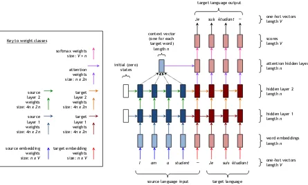
Figure 2: NMT architecture. This example has two layers, but our system has four. The different weight classes are indicated by arrows of different color (the black arrows in the top right represent simply choosing the highest-scoring word, and thus require no parameters). Best viewed in color.

tailed in Section 4.5, are corroborated by (Lu et al., 2016).

3 Our Approach

We first give a brief overview of Neural Ma-chine Translation before describing the model ar-chitecture of interest, the deep multi-layer recur-rent model with LSTM. We then explain the dif-ferent types of NMT weights together with our ap-proaches to pruning and retraining.

3.1 Neural Machine Translation

Neural machine translation aims to directly model the conditional probabilityp(y|x)of translating a source sentence, x1, . . . , xn, to a target sentence,

y1, . . . , ym. It accomplishes this goal through an

encoder-decoder framework (Kalchbrenner and Blunsom, 2013; Sutskever et al., 2014; Cho et al., 2014). Theencodercomputes a representation s

for each source sentence. Based on that source representation, the decoder generates a transla-tion, one target word at a time, and hence, decom-poses the log conditional probability as:

logp(y|x) =Xm

t=1logp(yt|y<t,s) (1) Most NMT work uses RNNs, but approaches differ in terms of: (a) architecture, which can

be unidirectional, bidirectional, or deep multi-layer RNN; and (b) RNN type, which can be Long Short-Term Memory (LSTM) (Hochreiter and Schmidhuber, 1997) or the Gated Recurrent Unit (Cho et al., 2014).

In this work, we specifically consider thedeep multi-layer recurrent architecture with LSTM as the hidden unit type. Figure 1 illustrates an in-stance of that architecture during training in which the source and target sentence pair are input for su-pervised learning. During testing, the target sen-tence is not known in advance; instead, the most probable target words predicted by the model are fed as inputs into the next timestep. The network stops when it emits the end-of-sentence symbol — a special ‘word’ in the vocabulary, represented by a dash in Figure 1.

3.2 Understanding NMT Weights

The source input sentence and target input sen-tence, represented as a sequence of one-hot vec-tors, are transformed into a sequence of word em-beddings by the embedding weights. These em-bedding weights, which are learned during train-ing, are different for the source words and the tar-get words. The word embeddings and all hidden layers are vectors of lengthn(a chosen hyperpa-rameter).

The word embeddings are then fed as input into the main network, which consists of two multi-layer RNNs ‘stuck together’ — an encoder for the source language and a decoder for the target lan-guage, each with their own weights. The feed-forward(vertical) weights connect the hidden unit from the layer below to the upper RNN block, and therecurrent(horizontal) weights connect the hid-den unit from the previous time-step RNN block to the current time-step RNN block.

The hidden state at the top layer of the decoder is fed through anattentionlayer, which guides the translation by ‘paying attention’ to relevant parts of the source sentence; for more information see (Bahdanau et al., 2015) or Section 3 of (Luong et al., 2015a). Finally, for each target word, the top layer hidden unit is transformed by the soft-maxweights into a score vector of lengthV. The target word with the highest score is selected as the output translation.

Weight Subgroups in LSTM – For the afore-mentioned RNN block, we choose to use LSTM as the hidden unit type. To facilitate our later discus-sion on the different subgroups of weights within LSTM, we first review the details of LSTM as for-mulated by Zaremba et al. (2014) as follows:

    i f o ˆ h    =     sigm sigm sigm tanh    T4n,2n

hl_t−1 hl

t−1

(2)

cl

t=f ◦clt−1+i◦ˆh (3)

hl

t=o◦tanh(clt) (4) Here, each LSTM block at timetand layerl com-putes as output a pair of hidden and memory vec-tors (hl

t, clt) given the previous pair (hlt−1, clt−1) and an input vector hl−1

t (either from the LSTM block below or the embedding weights ifl= 1). All of these vectors have lengthn.

The core of a LSTM block is the weight matrix

T4n,2nof size4n×2n. This matrix can be decom-posed into 8 subgroups that are responsible for the

interactions between {input gatei, forget gatef, output gateo, input signalˆh} × {feed-forward in-puthl_t−1, recurrent inputhl

t−1}. 3.3 Pruning Schemes

We follow the general magnitude-based approach of (Han et al., 2015b), which consists of pruning weights with smallest absolute value. However, we question the authors’ pruning scheme with re-spect to the different weight classes, and exper-iment with three pruning schemes. Suppose we wish to prune x% of the total parameters in the model. How do we distribute the pruning over the different weight classes (illustrated in Figure 2) of our model? We propose to examine three different pruning schemes:

1. Class-blind: Take all parameters, sort them by magnitude and prune thex% with smallest magnitude, regardless of weight class. (So some classes are pruned proportionally more than others).

2. Class-uniform: Within each class, sort the weights by magnitude and prune thex% with smallest magnitude. (So all classes have ex-actlyx% of their parameters pruned).

3. Class-distribution: For each classc, weights with magnitude less than λσc are pruned. Here,σcis the standard deviation of that class andλ is a universal parameter chosen such that in total,x%of all parameters are pruned. This is used by (Han et al., 2015b).

All these schemes have their seeming advantages. Class-blind pruning is the simplest and adheres to the principle that pruning weights (or equivalently, setting them to zero) is least damaging when those weights are small, regardless of their locations in the architecture. Class-uniform pruning and class-distribution pruning both seek to prune proportion-ally within each weight class, either absolutely, or relative to the standard deviation of that class. We find that class-blind pruning outperforms both other schemes (see Section 4.1).

3.4 Retraining

0 10 20 30 40 50 60 70 80 90 0

10 20

percentage pruned

BLEU

score

class-blind class-uniform class-distribution

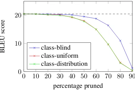
Figure 3: Effects of different pruning schemes.

weights are represented by zeros in the weight ma-trices, and we use binary ‘mask’ mama-trices, which represent the sparse structure of a network, to ig-nore updates to weights at pruned locations. This implementation has the advantage of simplicity as it requires minimal changes to the training and deployment code, but we note that a more complex implementation utilizing sparse matrices and sparse matrix multiplication could potentially yield speed improvements. However, such an im-plementation is beyond the scope of this paper.

4 Experiments

We evaluate the effectiveness of our pruning approaches on a state-of-the-art NMT model.1

Specifically, an attention-based English-German NMT system from (Luong et al., 2015a) is consid-ered. Training data was obtained from WMT’14 consisting of 4.5M sentence pairs (116M English words, 110M German words). For more details on training hyperparameters, we refer readers to Section 4.1 of (Luong et al., 2015a). All models are tested on newstest2014 (2737 sentences). The model achieves a perplexity of 6.1 and a BLEU score of 20.5 (after unknown word replacement).2

Whenretrainingpruned NMT systems, we use the following settings: (a) we start with a smaller learning rate of 0.5 (the original model uses a learning rate of 1.0), (b) we train for fewer epochs, 4 instead of 12, using plain SGD, (c) a simple learning rate schedule is employed; after 2 epochs, we begin to halve the learning rate every half an epoch, and (d) all other hyperparameters are the

1_{We thank the authors of (Luong et al., 2015a) for}

provid-ing their trained models and assistance in usprovid-ing the codebase athttps://github.com/lmthang/nmt.matlab.

2_{The performance of this model is reported under row}

global (dot)in Table 4 of (Luong et al., 2015a).

same, such as mini-batch size 128, maximum gra-dient norm 5, and dropout with probability 0.2. 4.1 Comparing pruning schemes

Despite its simplicity, we observe in Figure 3 that class-blind pruning outperforms both other schemes in terms of translation quality at all prun-ing percentages. In order to understand this result, for each of the three pruning schemes, we pruned each class separately and recorded the effect on performance (as measured by perplexity). Figure 4 shows that with class-uniform pruning, the over-all performance loss is caused disproportionately by a few classes: target layer 4, attention and soft-max weights. Looking at Figure 5, we see that the most damaging classes to prune also tend to be those with weights of greater magnitude — these classes have much larger weights than others at the same percentile, so pruning them under the class-uniform pruning scheme is more damaging. The situation is similar for class-distribution pruning.

By contrast, Figure 4 shows that under class-blind pruning, the damage caused by pruning soft-max, attention and target layer 4 weights is greatly decreased, and the contribution of each class to-wards the performance loss is overall more uni-form. In fact, the distribution begins to reflect the number of parameters in each class — for ex-ample, the source and target embedding classes have larger contributions because they have more weights. We use only class-blind pruning for the rest of the experiments.

Figure 4 also reveals some interesting informa-tion about the distribuinforma-tion of redundancy in NMT architectures — namely it seems that higher lay-ers are more important than lower laylay-ers, and that attention and softmax weights are crucial. We will explore the distribution of redundancy further in Section 4.5.

4.2 Pruning and retraining

Pruning has an immediate negative impact on per-formance (as measured by BLEU) that is exponen-tial in pruning percentage; this is demonstrated by the blue line in Figure 6. However we find that up to about 40% pruning, performance is mostly un-affected, indicating a large amount of redundancy and over-parameterization in NMT.

im-source layer

1

source layer

2

source layer

3

source layer

4

target layer

1

target layer

2

target layer

3

target layer

4

attention softmax

source

embedding target

embedding

0 5 10 15

perple

xity

change

class-blind class-uniform class-distribution

Figure 4: ‘Breakdown’ of performance loss (i.e., perplexity increase) by weight class, when pruning 90% of weights using each of the three pruning schemes. Each of the first eight classes have 8 million weights, attention has 2 million, and the last three have 50 million weights each.

0 0.1 0.2 0.3 0.4 0.5

100

101

magnitude of largest deleted weight

perple

xity

change

Figure 5: Magnitude of largest deleted weight vs. perplexity change, for the 12 different weight classes when pruning 90% of parameters by class-uniform pruning.

proved upon, up to 80% pruning (20.91 BLEU), with only a small performance loss at 90% pruning (20.13 BLEU). This may seem surprising, as we might not expect a sparse model to significantly out-perform a model with five times as many pa-rameters. There are several possible explanations, two of which are given below.

Firstly, we found that the less-pruned models perform better on the training set than the vali-dation set, whereas the more-pruned models have closer performance on the two sets. This indicates that pruning has a regularizing effect on the re-training phase, though clearly more is not always better, as the 50% pruned and retrained model has better validation set performance than the 90%

0 10 20 30 40 50 60 70 80 90 0

10 20

percentage pruned

BLEU

score

pruned

pruned and retrained sparse from the beginning

Figure 6: Performance of pruned models (a) after pruning, (b) after pruning and retraining, and (c) when trained with sparsity structure from the out-set (see Section 4.3).

pruned and retrained model. Nonetheless, this reg-ularization effect may explain why the pruned and retrained models outperform the baseline.

0 1 2 3 4 5

·105

2 4 6 8

training iterations

loss

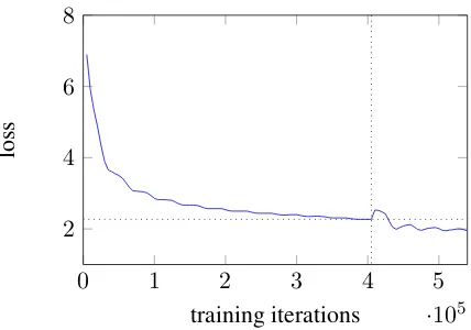
Figure 7: The validation set loss during training, pruning and retraining. The vertical dotted line marks the point when 80% of the parameters are pruned. The horizontal dotted line marks the best performance of the unpruned baseline.

pruning is beneficial in the long-run.

4.3 Starting with sparse models

The favorable performance of the pruned and re-trained models raises the question: can we get a shortcut to this performance by starting with sparse models? That is, rather than train, prune, and retrain, what if we simply prune then train? To test this, we took the sparsity structure of our 50%–90% pruned models, and trained completely new models with the same sparsity structure. The purple line in Figure 6 shows that the ‘sparse from the beginning’ models do not perform as well as the pruned and retrained models, but they do come close to the baseline performance. This shows that while the sparsity structure alone contains useful information about redundancy and can therefore produce a competitive compressed model, it is im-portant to interleave pruning with training.

Though our method involves just one pruning stage, other pruning methods interleave pruning with training more closely by including several iterations (Collins and Kohli, 2014; Han et al., 2015b). We expect that implementing this for NMT would likely result in further compression and performance improvements.

4.4 Storage size

The original unpruned model (a MATLAB file) has size 782MB. The 80% pruned and retrained model is 272MB, which is a 65.2% reduction. In this work we focus on compression in terms of number of parameters rather than storage size,

be-cause it is invariant across implementations.

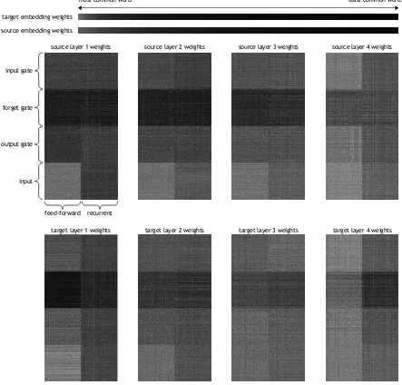
4.5 Distribution of redundancy in NMT We visualize in Figure 8 the redundancy struc-tore of our NMT baseline model. Black pix-els represent weights near to zero (those that can be pruned); white pixels represent larger ones. First we consider the embedding weight matrices, whose columns correspond to words in the vocab-ulary. Unsurprisingly, in Figure 8, we see that the parameters corresponding to the less common words are more dispensable. In fact, at the 80% pruning rate, for 100 uncommon source words and 1194 uncommon target words, we delete all

parameters corresponding to that word. This is not quite the same as removing the word from the vocabulary — true out-of-vocabulary words are mapped to the embedding for the ‘unknown word’ symbol, whereas these ‘pruned-out’ words are mapped to a zero embedding. However in the original unpruned model these uncommon words already had near-zero embeddings, indicating that the model was unable to learn sufficiently distinc-tive representations.

Returning to Figure 8, now look at the eight weight matrices for the source and target connec-tions at each of the four layers. Each matrix corre-sponds to the4n×2nmatrixT4n,2nin Equation (2). In all eight matrices, we observe — as does (Lu et al., 2016) — that the weights connecting to the input ˆh are most crucial, followed by the in-put gate i, then the output gateo, then the forget gatef. This is particularly true of the lower lay-ers, which focus primarily on the input ˆh. How-ever for higher layers, especially on the target side, weights connecting to the gates are as important as those connecting to the inputˆh. The gates repre-sent the LSTM’s ability to add to, delete from or retrieve information from the memory cell. Figure 8 therefore shows that these sophisticated memory cell abilities are most important at theendof the NMT pipeline (the top layer of the decoder). This is reasonable, as we expect higher-level features to be learned later in a deep learning pipeline.

target embedding weights

source embedding weights

least common word most common word

source layer 1 weights

recurrent feed-forward

input gate

forget gate

output gate

input

source layer 2 weights source layer 3 weights source layer 4 weights

target layer 1 weights target layer 2 weights target layer 3 weights target layer 4 weights

use of the higher-level representation of the sen-tence so far (the recurrent input).

Lastly, on close inspection, we notice several white diagonals emerging within some subsquares of the matrices in Figure 8, indicating that even without initializing the weights to identity ma-trices (as is sometimes done (Le et al., 2015)), an identity-like weight matrix is learned. At higher pruning percentages, these diagonals be-come more pronounced.

5 Generalizability of our results

To test the generalizability of our results, we also test our pruning approach on a smaller, non-state-of-the-art NMT model trained on the WIT3 Vietnamese-English dataset (Cettolo et al., 2012), which consists of 133,000 sentence pairs. This model is effectively a scaled-down version of the state-of-the-art model in (Luong et al., 2015a), with fewer layers, smaller vocabulary size, smaller hidden layer size, no attention mechanism, and about 11% as many parameters in total. It achieves a BLEU score of 9.61 on the validation set.

Although this model and its training set are on a different scale to our main model, and the lan-guage pair is different, we found very similar re-sults. For this model, it is possible to prune 60% of parameters with no immediate performance loss, and with retraining it is possible to prune 90%, and regain original performance. Our main observa-tions from Secobserva-tions 4.1 to 4.5 are also replicated; in particular, class-blind pruning is most success-ful, ‘sparse from the beginning’ models are less successful than pruned and retrained models, and we observe the same patterns as seen in Figure 8.

6 Future Work

As noted in Section 4.3, including several itera-tions of pruning and retraining would likely im-prove the compression and performance of our pruning method. If possible it would be highly valuable to exploit the sparsity of the pruned mod-els to speed up training and runtime, perhaps through sparse matrix representations and mul-tiplications (see Section 3.4). Though we have found magnitude-based pruning to perform very well, it would be instructive to revisit the orig-inal claim that other pruning methods (for ex-ample Optimal Brain Damage and Optimal Brain Surgery) are more principled, and perform a com-parative study.

7 Conclusion

We have shown that weight pruning with retrain-ing is a highly effective method of compression and regularization on a state-of-the-art NMT sys-tem, compressing the model to 20% of its size with no loss of performance. Though we are the first to apply compression techniques to NMT, we obtain a similar degree of compression to other current work on compressing state-of-the-art deep neural networks, with an approach that is simpler than most. We have found that the absolute size of pa-rameters is of primary importance when choosing which to prune, leading to an approach that is ex-tremely simple to implement, and can be applied to any neural network. Lastly, we have gained insight into the distribution of redundancy in the NMT architecture.

8 Acknowledgment

References

M Gethsiyal Augasta and T Kathirvalavakumar. 2013. Pruning algorithms of neural networks - a compara-tive study. Central European Journal of Computer Science, 3(3):105–115.

Dzmitry Bahdanau, Kyunghyun Cho, and Yoshua Ben-gio. 2015. Neural machine translation by jointly learning to align and translate. InICLR.

Mauro Cettolo, Christian Girardi, and Marcello Fed-erico. 2012. Wit3_{: Web inventory of transcribed} and translated talks. InEAMT.

Wenlin Chen, James T Wilson, Stephen Tyree, Kilian Q Weinberger, and Yixin Chen. 2015. Compressing neural networks with the hashing trick. InICML. Kyunghyun Cho, Bart van Merrienboer, Caglar

Gul-cehre, Fethi Bougares, Holger Schwenk, and Yoshua Bengio. 2014. Learning phrase representations using RNN encoder-decoder for statistical machine translation. InEMNLP.

Maxwell D Collins and Pushmeet Kohli. 2014. Mem-ory bounded deep convolutional networks. arXiv preprint arXiv:1412.1442.

Matthieu Courbariaux, Yoshua Bengio, and Jean-Pierre David. 2015. Low precision arithmetic for deep learning. InICLR workshop.

Emily L Denton, Wojciech Zaremba, Joan Bruna, Yann LeCun, and Rob Fergus. 2014. Exploiting linear structure within convolutional networks for efficient evaluation. InNIPS.

Suyog Gupta, Ankur Agrawal, Kailash Gopalakrish-nan, and Pritish Narayanan. 2015. Deep learning with limited numerical precision. InICML.

Song Han, Huizi Mao, and William J Dally. 2015a. Deep compression: Compressing deep neural net-works with pruning, trained quantization and huff-man coding. InICLR.

Song Han, Jeff Pool, John Tran, and William Dally. 2015b. Learning both weights and connections for efficient neural network. InNIPS.

Babak Hassibi and David G Stork. 1993. Second or-der or-derivatives for network pruning: Optimal brain surgeon. Morgan Kaufmann.

Geoffrey Hinton, Oriol Vinyals, and Jeff Dean. 2015. Distilling the knowledge in a neural network. In NIPS Deep Learning Workshop.

Sepp Hochreiter and J¨urgen Schmidhuber. 1997. Long short-term memory. Neural computation, 9(8):1735–1780.

Forrest N Iandola, Matthew W Moskewicz, Khalid Ashraf, Song Han, William J Dally, and Kurt Keutzer. 2016. Squeezenet: Alexnet-level accuracy with 50x fewer parameters and<1mb model size. arXiv preprint arXiv:1602.07360.

Max Jaderberg, Andrea Vedaldi, and Andrew Zisser-man. 2014. Speeding up convolutional neural net-works with low rank expansions. InNIPS.

S´ebastien Jean, Kyunghyun Cho, Roland Memisevic, and Yoshua Bengio. 2015a. On using very large target vocabulary for neural machine translation. In ACL.

S´ebastien Jean, Orhan Firat, Kyunghyun Cho, Roland Memisevic, and Yoshua Bengio. 2015b. Montreal neural machine translation systems for WMT’15. In WMT.

Nal Kalchbrenner and Phil Blunsom. 2013. Recurrent continuous translation models. InEMNLP.

Quoc V Le, Navdeep Jaitly, and Geoffrey E Hin-ton. 2015. A simple way to initialize recurrent networks of rectified linear units. arXiv preprint arXiv:1504.00941.

Yann Le Cun, John S Denker, and Sara A Solla. 1989. Optimal brain damage. InNIPS.

Zhouhan Lin, Matthieu Courbariaux, Roland Memise-vic, and Yoshua Bengio. 2016. Neural networks with few multiplications. InICLR.

Zhiyun Lu, Vikas Sindhwani, and Tara N Sainath. 2016. Learning compact recurrent neural networks. InICASSP.

Minh-Thang Luong and Christopher D. Manning. 2015. Stanford neural machine translation systems for spoken language domain. InIWSLT.

Minh-Thang Luong and Christopher D. Manning. 2016. Achieving open vocabulary neural machine translation with hybrid word-character models. In ACL.

Minh-Thang Luong, Hieu Pham, and Christopher D Manning. 2015a. Effective approaches to attention-based neural machine translation. InEMNLP.

Minh-Thang Luong, Ilya Sutskever, Quoc V Le, Oriol Vinyals, and Wojciech Zaremba. 2015b. Address-ing the rare word problem in neural machine trans-lation. InACL.

Kenton Murray and David Chiang. 2015. Auto-sizing neural networks: With applications to n-gram lan-guage models. InEMNLP.

Rohit Prabhavalkar, Ouais Alsharif, Antoine Bruguier, and Ian McGraw. 2016. On the compression of re-current neural networks with an application to lvcsr acoustic modeling for embedded speech recognition. InICASSP.

Suraj Srinivas and R Venkatesh Babu. 2015. Data-free parameter pruning for deep neural networks. In BMVC.

Ilya Sutskever, Oriol Vinyals, and Quoc V. Le. 2014. Sequence to sequence learning with neural net-works. InNIPS.