II. AUTOMATED ASSEMBLY

(1)



ABSTRACT - Modern manufacturing systems mainly consist of processes and machines. Simulating an assembly process requires input from the production processes and this requires a detailed study of a given manufacturing environment. Most research has been concentrating on getting input from and simulating specific assembly processes. Assembly processes can be grouped into assembly families from which a simulation procedure/program can be designed. This procedure/program can be applied to this family of assembly processes based on the products, e.g. automotive assembly products. This paper envisages creating a generic assembly program that can be used to simulate a given family of assembly processes. This family of products comprises of assembling of all types of motor assembly processes within their given families.

I. INTRODUCTION

Automated assembly is a complex manufacturing system in which products are manufactured from a number of components [2]. Products are made from different materials and require flexible and precise mechanisms, which are computer controlled. The assembly process make use of robots, AGVs, etc equipped with highly accurate sensory systems [3].

II. AUTOMATEDASSEMBLY

Automation process includes the coordination of design and manufacturing activities between many and among supplies of assembly components/parts. Assembly process involves a number of operations, which require assembling together thousands of fabricated and purchased components/parts, subassemblies and systems-coordination. Purchased components are outsourced from many suppliers who generally use different data formats, which are not usually compatible. Yet this data must be shared among many of these companies involved in the production process.

III. TYPICALAUTOMATEDASSEMBLY

This is a system for assembling a series of parts movable along the guided track in an assembly area. The system consists of a work station and this station could be having program-controlled robot or automatic guided vehicles (AGVs). There is also a buffer area for storing sets of parts within the work station. This work station will assembly each set of parts into an assembly, unload the assembly into the guide path or conveyor, which leads to another work station. A conveyor or AGVs systems are the transport systems of an assembly plant. For the conveyor system, the assembly will be stopping in predetermined positions relative to the guided assembly and unload stations/points. Sometimes the work stations are along the conveyor belt.

T. Sithebe is with University of South Africa (UNISA), South Africa (email: [email protected])

IV. TRANSPORTSYSTEM

The robots and transport systems are computer controlled so that these robots or AGVs can pick and place the given sets of parts and perform other functions such as welding during motion from station to station until the assembly process is completed. The assembly process contains a plurality of knitting stations and storage buffer area. Each of these stations is located along the guide path or the conveyor. The control means automatically monitor and coordinate operations of each robot with the automatic transferring of the assembly to and from the work stations to control the flow of parts and pallets in the assembly area. In an event of failure of a robot the control means automatically redistributes any remaining work of the failed robot [5].

V. AUTOMATIONCONCEPT

The appropriate automation concepts are achieved with innovative and well proven products and systems through close cooperation with customers. Function of the system, economy, schedule and delivery liability and high availability being the main focus. Automation can also be associated with the “digital factory” with its largely stand alone and holistic facilities from the press shop, body shop, power train shop, paint shop to the trim shop (general automotive assembly shop).

VI. LITERATUREONASSEMBLY

For a given family of Automation, there is a need for a generic approach that encompasses this family. This approach will culminate in a simulation program that can be used for the assessment of this group of families, and establish or evaluate the performance of this process or of an existing process. This can be made in the form of standard software for a given family of manufacturing processes and products. A generic simulation model concept has been applied to “Software Interoperability” by Deogratias Kibira and Charles R. Mclean (2007) [1]. They introduced a Generic Simulation of Automotive Assembly for Interoperability Testing. Their simulation was meant for a specific sector of an assembly process and environment.

A generic modeling system for automated mechanical assembly (1980), [2] was developed by M. A. Wesley. T. Lzano-Perez, L. I. Liberman, M. A. Lavin and D. D. Grossman. They described a language or a technique for the geometric and physical properties for mechanical assembly parts. This technique look at properties of 3-D objects including parts, tools and the assembler itself. This results in a data base in which objects and assemblies are represented by nodes in a graph structure, with the edges of the graph representing relationships among the objects, such as attachments, constraint and assembly. This has found some application in automotive assembly since its publication. It is

Generic Simulation

(2)

however necessary to look further than mechanical assembly and broaden this family as there are changes in automated assembly that needs to be considered.

The “Automated process planning assembly for printed circuit card assembly” by L. F. McHinns, J. C. Ammons, M. Carlyle, L Cranmer, G. W. Deuy, K. P. Ellis, C. A. Tovey and H. Xu (1992) [3]. They looked at the circuit assembly process. This in itself is a family of circuit card, these have a wide application. The framework however can be applied as an approach to other assembly processes giving the decision hierarchy of that family of products.

K. Lee and D. C. Gossard looked at a hierarchical data structure for representing assemblies (1985) [4]. Using CAD, they assessed the data structure used to store topological and geometrical information on each component in an assembly. Then they looked at data structure used to store information on how all the components in an assembly are connected. This gives a tree structure linking all the parts together. The “Generic flexible assembly system design” by N. F. Edmondson and A. H. Redford [5], involves the design, selection and integration of different mechanical systems in order to develop an assembly system which is capable of assembling a variety of products having an unknown specification. Their system configuration is dependent on a variety of factors such as product size, weight, and component insertion direction and manipulator geometry. Then a novel generic assembly system is formulated.

VII. OBJECTIVESOFTHISPAPER

Whilst all these researchers had in their work some form of generic approach, it is imperative to have a generic approach with a pre-defined family of products, selected range of tools and a limited number of work-stations. This assembly system will culminate with a simulation for use to assess the performance of a selected process.

This paper envisages establishing a generic simulation process, which will be based on the generic algorithm and generic assumptions to be used to simulate an automated assembly process with the main one being an automated assembly.

VIII. GENERIC MULTI WORK-STATION DIAGRAM

Where BS stands for Buffer storage areas, and are subdivided according to the given sequence of assembly per work-station. WS stands for work-station.

The diagram above is a layout of the assembly work-stations. The number of work-stations (n) is up to ten for this program.

The work-stations follow one another and the buffer storage material is located on each work-station. There is an independent assembly order for each work-station.

IX. FLOWCHART

Where

j



1 ,

2 ,

3 ,...

m

and

j



i

k



n

. Given that

i

k is

the component of the given product and

k

is the identification factor according to the assembly process. Once identified, the component will be transferred to the assembler, and if the assembler has secured the component, and requires the next, it will send a signal



_k. Where



W S 1

W S 2

W S 3

W S n

BS1 BS2 BS3 BS n

Direction of

Assembly process Conveyor

belt

Comp

j

i

_k



entry

Identify comp

i

_k



j



1

Has comp

1 



j

i

_k been

identified? _No

Yes

Transfer comp

i

_k



j



1

to Assembler

Has comp

1 



j

i

k been

transferred to assembler?

Yes

No

Assemble comp

j

i

_k



with comp

i

_k



j



1

Have the comp been assembled?

No

Yes

Identify comp

i

_k



n

Has comp

n

i

_k



been

identified? No

Yes

Transfer comp

i

_k



n

to Assembler

Has comp

n

i

_k



been transferred to

assembler? No

Assemble comp

n

i

k



with

assembly

Repeat the loop until

10 

n

(3)

relates to the success or failure of the operation during the assembly process and

k

identifies which component comes next. It will be repeated until the assembly process is complete.

X EXCEL SPREADSHEET

The excel spreadsheet is the platform from which to control and input the values according to given plant requirements. In this spreadsheet, one can select the number of work-stations, number of components per work-station and the availability of component or parts to a work-station. In the program there are a total of ten work-stations. All the work-stations are along the conveyor. In each work-station there are a total of up to four components which can be assembled. All changes in the program are carried-out on the excel spreadsheet.

Work Stat Componen% AvailabiMin Average Max Min Average Max

1 100 5 7 10 1 3 5 10

2 100 5 7 10 2 3 5

3 100 5 7 10 2 3 5

4 100 5 7 10 2 3 5

5 100 5 7 10 0 1 1

6 100 5 7 10 0 1 1

7 100 5 7 10 0 1 1

8 100 5 7 10 0 1 1

9 100 5 7 10 2 4 6

10 100 5 7 10 2 4 6

11 100 5 7 10 2 4 6

12 100 5 7 10 2 4 6

3

Delay Time (Minutes) Assembly Time (Minutes) Number of Work

1

2

The components or parts are varied according to their availability. An availability of 100 percent implies that the components are readily available, but if the components are outsourced, the availability can be adjusted to suit the source. XI ARENA PROGRAM

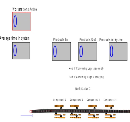
Work Station 1

Component 1 Component 2 Component 3 Component 4

Wait For Work Station 1 to Finish Before Releasing Next Unit

Average time in system _{Products In} _{Products Out} _{Products in System}

Workstations Active

Hold if Conveying Lags Assembly

Hold if Assembly Lags Conveying

0

_{0 0}

₀

0

The diagram above shows the number of active work-stations, average time of components in the system, number of components in and out of the Assembly process.

Shown here is work-station 1, which is similar in setup to all others.

XI RESULTS CATEGORY OVERVIEW

Generic Assembly one

[image:3.595.47.294.264.411.2] [image:3.595.305.548.393.734.2]

Replications: 3 Time units: minutes Table 1

This table shows the usage of the conveyor belt. The figures in the table outlines the times during which the conveyor is in use. Utilisation of the conveyor is also indicated in te second part of the table.

Bloc ked

Ave Half widt h

Min average

Max ave

Min value

Max value

Conv eyor 1

0.2955 0.00 0.2948 0.2968 0.00 1.0000

Utilization Conv eyor 1

0.0290 0190

0.00 0.028999 32

0.029005 66

0.00 0.0314 2857

These are the activities pertaining to the utilization of the conveyor.

Entity (Components) Table 2

The table below traces the activities encompassing entity 1 (or component 1) during the assembly process. This table shows the amount of time during which the component is in the assembly process.

VA Time

Ave Half widt h

Min ave Max ave Min

value Max value

Entity 1

13.05 86

0.02 13.0514 013.068 7

0.00 22.256 3 NVA

Time Entity 1

0.00 0.00 0.00 0.00 0.00 0.00

Wait time Entity 1

11.41 94

0.02 11.4108 11.4298 0.00 28.779 9 Transf

er Time Entity 1

8.288 0.01 8.283 8.393 1.00 23.256

3 Total

Time Entity 1

32.76 6

0.05 32.7452 32.7865 10.35 26

48.226 2

Other

Ave Half

width Min ave

Max ave

Min value

Max value Number in

Entit y 1

81983. 33

135.40 81929.0 81038.0

Number out Entit y 1

81966. 33

124.42 81918.0 82018.0

WIP Entit y 1

18.653 1

0.00 18.6528 18.6535 0.00 21.0

0

[image:3.595.47.294.491.723.2]

(4)

This table shows no activity in the given components. These components are from those work-stations which are idle. A queue is the activity relating to work-in-progress.

[image:4.595.308.546.54.763.2]

The next table relates to work-in-progress of components in those work-station in which assembling is in progress. The next table also shows the activities between the conveyor and work-stations. This shows the times at which the work-station is idle having completed an assembly process. Table 3 Waiting time

Queue or work-in-progress shown in the tables below reflects the activities within the workstation and shows the number of components in these queues.

Ave Half

width Min ave Max ave Min value Max value Hold at the

end of station. Queue

8.9899 0.06 8.9650 9.01

61 4.46 35

13.9 344

Hold at the end of station10. Queue 11.998 5 0.03 11.986 1 12.0 135 6.35 26 18.0 458

Hold at the end of station9. Queue 12.000 2 0.05 11.981 0 12.0 194 0.06 7078 84 3.31 67 Hold until finished converying2. Queue

1.3297 0.01 19.298

0 19.3 226 11.2 904 28.7 799

WS1 Ready for next assembly? Queue

Table 4 Number waiting

In this table both the half width and the minimum value are 0.00. This is the time during which the components are held at a workstation awaiting the completion of preceding assembly process. These are the performances of machines in a workstation.

Average Min

ave

Max ave

Max value Hold at the

end of station. Queue

0.00 0.00 0.00 0.00

Hold at the end of

0.6206 0.4642 0.4666 1.0000

station10. Queue Hold at the end of station2. Queue

0.00 0.00 0.00 0.00

Hold at the end of station3. Queue

0.6215 0.6203 0.6223 1.0000

0.6212 0.6206 0.6221 1.0000

0.6208 0.6195 0.6216 1.0000

0.6203 0.6296 0.6209 1.0000

0.6211 0.6200 0.6220 1.0000

0.6207 0.6201 0.6212 1.0000

0.06207 0.6193 0.6217 1.0000

Hold until finished conveying2 Queue

0.06884919 0.06858248 0.06911106 1.0000

Hold until finished conveying3. Queue

0.00 0.00 0.00 0.00

Hold until finished conveying. Queue

0.00 0.00 0.00 0.00

WS1 Ready for next assembly? Queue

[image:4.595.41.290.216.621.2]

(5)

[image:5.595.55.557.73.795.2]

The next table shows the activities relating to the active work-stations.

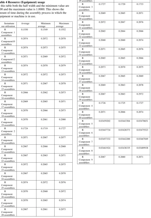
Table 4 Resource (Equipment) usage

In this table both the half width and the minimum value are 0.00 and the maximum value is 1.0000. This shows the amount of time during the assembly process in which the equipment or machine is in use.

Instantane ous utilisation

Average Minimum average

Maximum average R

Component 1 assemblers

0.1550 0.1549 0.1552

R Component10 assemblers

0.2074 0.2072 0.2078

R Component 11 assemblers

0.2074 0.2073 0.2075

R Component12 assemblers

0.2071 0.2069 0.2072

0.2074 0.2070 0.2079

0.2072 0.2072 0.2073

0.2071 0.2067 0.2078

0.2066 0.2062 0.2073

0.2069 0.2065 0.2071

0.2070 0.2066 0.2073

0.2070 0.2061 0.2080

0.1724 0.1719 0.1727

0.2071 0.2067 0.2077

0.2067 0.2066 0.2068

0.2067 0.2063 0.2071

0.2072 0.2065 0.2075

0.2067 0.2065 0.2070

0.2074 0.2072 0.2076

0.2070 0.2068 0.2072

0.2070 0.2065 0.2074

0.2067 0.2061 0.2073

0.2069 0.2066 0.2091

0.1727 0.1720 0.1733

0.2069 0.2065 0.2071

0.2072 0.2067 0.2076

0.2065 0.2064 0.2066

0.2068 0.2060 0.2074

0.2071 0.2065 0.2076

0.2065 0.2065 0.2066

0.2073 0.2070 0.2075

0.2067 0.2065 0.2069

0.2069 0.2063 0.2078

0.2067 0.2063 0.2972

0.1726 0.1725 0.1727

0.2071 0.2066 0.2074

0.03459202 0.03443304 0.03470651

0.03447734 0.03428373 0.03475523

0.03457332 0.03442200 0.03467049

0.03461924 0.03438335 0.03489938

(6)

[image:6.595.47.255.55.215.2] [image:6.595.49.258.320.478.2]

Figure 1: the usage of machines within the workstation This figure outlines the usage of machines within the workstation. This can be customized to suit specific machines within a given workstation, and each machine can be monitored based on the indicated performance in such a table.

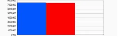
Figure 2: the performance on machines within a workstation under different conditions

[image:6.595.51.243.578.638.2]

As in figure 1, figure 2 shows the performance on machines within a workstation under different conditions. Machines can be assessed in different operating conditions so that come-up with an appropriate usage of a workstation.

Figure 3: the utilization of work-stations currently in use. A resource is a work-station, conveyor or the transport system; it is thus a component of the assembly process.

XII CONCLUSION

After each run one can then generate reports which include the utilisation of each workstation, number of components used, and number of products or assemblies. These reports will be used to assess the performance of a given plant or assembly process.

This work gives Managers and Engineers the easy access to crucial production information of a manufacturing process. This information can then be utilised to optimise the manufacturing processes, and reduce costs of system design as this is simulated before implementation.

ACKNOWLEDGMENT

Professor Z. Katz from the University of Johannesburg has played a greatest role in the success of this paper.

REFERENCES

[1]. Generic Simulation of Automotive Assembly for Interoperability Testing. Proceedings of the 2007 Winter Simulations Conference. S. G. Henderson, B. Biller, M. H. Heish, J. Shortle, J. D. Tew and R.R. Barton

[2]. A geometric modeling system for automated mechanical assembly by M. A. Wesley, T. Lozano-Perez, L. I. Lieberman, M. A. Lavin and D. D. Grossman. IBM Journal of Research and Development, 1980.

[3]. Automated process planning for printed circuit assembly by L. F. McGinnis, J. C. Ammons, M. Carlyle, L. Cranmer, G. W. Depuy, K. P. Ellis, C. A. Tovey and H. Xu. 1992.

[4]. A hierarchical data structure for representing assemblies by Kunwoo Lee and David C. Gossard, 1985. Computer-aided Design Volume 17.

[5]. Generic flexible assembly system design by N. F. Edmondson and A. H. Redford, Assembly Automation, volume 22, 2002.

[6]. A Dynamic Algorithm for the Control of Automotive Painted Body Storage. Dug Hee Moon, Cheng Song and Lee Hoon Ha. SIMULATION 2005;81;773

[7]. An automated assembly system for a microasembly station, by A. Mardanov, J. Seyfried and S. Fatikow. Institue for Process Control and Robotics, University of Karlsruhe, Kaiserstr, Karlsuhe, Germany. Ufa State Aviation Technical University, Department of Technical Cybernetics, Bashkortostan, Russian Federation

[8]. Modelling Strain of Manual Work in Manufacturing Systems. Proceedings of the 1994 Winter Simulation Conference by J. D. Manivannan, D. A. Sadowski and A. F. Seila.

[9]. Method for automated assembly of assemblies such as automotive assemblies and system utilizing same, by Anthony R. and Haba, Jr. et al.

[10].Simulation modeling and analysis of a new mixed model production lines. Proceedings of the 2005 Winter Simulation Conference. By M. E. Kuhl, N. M. Steiger, F. B. Armsrong and J. A. Joines.

[11].Simulation-aided design of production and assembly cells in an automotive company.