Abstract—Short term load forecasting (STLF), which aims to predict system load over an internal of one day or one week, plays a crucial role in the control and scheduling operations of a power system. Most existing techniques on short term load forecasting try to improve the performance by selecting different prediction models. However, the performance also rely heavily on the quality of training data. This paper proposes a novel short term load forecasting approach based on training data selection. There are two main characteristics of the proposed method that distinguish it from the previous studies. The first characteristic is that the load curve of a time interval before the target hour is regard as the benchmark of training data instead of the cluster center of all historical data used in previous studies. The second characteristic is the load curves are normalized for comparison to the benchmark. Thus the load curves having similar trend with the benchmark can be selected for training. Experiments conducted on the real load data show significant improvement over the baseline method.
Index Terms—Short Term Load Forecasting, Training Data Selection, Load Curve Analysis
I. INTRODUCTION
OAD forecasting, which anticipates the future load by analyzing the historical data, plays a crucial role in the efficient planning, operation and maintenance of a power system. Short term load forecasting (STLF), which aims to predicts system load over an internal of one day or one week, is necessary for the control and scheduling operations of a power system. Further analyses such as load flow are also based on the results of the short term load forecasting.
Generally speaking, prediction model selection and training data selection are two issues which should be considered in load forecasting. Most existing techniques on short term load forecasting try to improve the performance by selecting different prediction models, such as linear regression[1], exponential smoothing, stochastic process, auto-regressive and moving average (ARMA) models[2], data mining models, and the widely used artificial neural networks (ANN)[3,4]. However, different models suffer from different problems. Linear regression does not perform well due to the lack of self-learning capability. Furthermore, weather changes cannot be easily integrated in linear regression models. In time series methods, load data are regard as cyclical time series changed by season, week, day or hour. Auto-regressive (AR) models, moving average (MA) models
Manuscript received December 8, 2010; revised January 11, 2011. Y. Yang, Y. Meng, Y. Xia, Y. Lu, and H. Yu are with the Fujitsu Research & Development Center Co., LTD. 15/F, Tower A, Ocean International Center,No.56 Dong Si Huan Zhong Rd, Chaoyang District, Beijing, 100025, P.R. China (phone: +86-10-59691000 ext 5752; fax: +86-10-59691504; e-mail: [email protected]).
and ARMA are typical time series methods which have been widely used for load forecasting. But time series methods, which are vulnerable to dirty data, rely heavily on the quality and size of historical data. In the recent studies, the ANN has been popular used for short term load forecasting with satisfactory results. Since the input variables of ANN are difficult to be selected, choosing appropriate training data becomes crucial in ANN based STLF methods.
As a result, some previous studies concentrate on selecting historical data for training. Fuzzy logic and case-based reasoning (CBR) are applied to depict different clusters of days[5]. According to the usage of weather changes, STLF techniques can be divided into three major groups[6]: non-weather sensitive models, weather-sensitive models, and hybrid models. Most similar day selection based STLF methods, which consider weather variables (such as temperature and humidity) and day type, are weather-sensitive. The methods using the day type information are straight forward. For an instance, the load curves of Friday may be collected from historical data in order to predict the load curve of next Friday. Thus not so many techniques can be applied. Instead, most related studies concentrate on the weather information based algorithms. Load is closely related to the weather changes. But weather is not the only factor which leads to load changes. Load curves themselves are the most direct way to characterize the abnormal days. However, load curves, which have a greater impact on load forecasting, are rarely considered in recent studies. Existing techniques always divides historical data into pieces according to different days. After division, load curves of particular days are used for training. The last 24 hour load information is often used to predict the next hour load. For an instance, when the selected model predicts the load of 7:00 am of a given day. The last 24 hour load data before this hour, which is from 7:00 am of the day before the given day to 6:00 am of the day, is used for prediction. The load data of the same hours (7:00 am – 6:00 am) are utilized to train the selected prediction model. Generally speaking, the same hours of similar days are likely to have similar trend. However, some other load curves of different hours may also similar and useful for the prediction, such as (8:00 am – 7:00 am) and (6:00 am – 5:00 am) of particular days in this case. This situation was rarely considered in previous studies.
In this paper, a novel approach is proposed for short term load forecasting. The proposed approach aims to select more appropriate training data in order to achieve satisfied performance. Compared to the previous studies, the load curve of a time interval before the target hour is regard as the benchmark of training data instead of the cluster center of all historical data. It makes more sense to select similar data for training and forecasting. Second, the approach selects similar
An Efficient Approach for Short Term Load
Forecasting
Yuhang Yang, Yao Meng, Yingju Xia, Yingliang Lu, and Hao Yu
load curves from the whole time series of all the historical load data instead of choosing training data from load curves of pre-divided single days. More candidates are obtained by using all the sub time series of the same time interval instead of load curves of the same hours. Thus more appropriate training data can be selected for STLF by analyzing historical load curves. Experiments are conducted on the real load data to verify the efficiency of the approach. The proposed approach can work by using only historical load curves if the weather information are not available. On the other hand, weather information can be easily integrated in the model. Thus the performance can be further improved by using more information.
The rest of the paper is organized as follows. Section 2 describes the proposed algorithms. Section 3 explains the experiments and the performance evaluation. Section 4 is the conclusion.
II. ALGORITHM DESIGN
As described in Section 1, training data selection is important for short term load forecasting. The main purpose of the proposed approach is to select more appropriate load curves for training in order to achieve satisfactory forecasting results. Thus the accuracy of load forecasting could be improved by using more appropriate training data. Some previous studies have been done on training data selection. The typical selection process is as follows. First, the historical load curve is divided into pieces according to the time interval used to predict the load of next hour. Second, the cluster center of all the divided load curves is obtained. Third, the distance between each load curve and the cluster center is measured and the abnormal ones (the load curves having long distances to the cluster center) are filtered out. Such algorithms suffer from two problems. The first problem is that the load of the target hour and the load curve before that may be not similar to the most of historical data. Thus selecting the most common data for training is not the best solution. The second problem is that only the load curves of the same hours in different days are taken as candidates for training. Many other similar load curves may be not included. This study proposes a novel approach in order to overcome such problems. There are two main characteristics of the proposed method that distinguish it from the previous studies. The first characteristic is that the load curve of a time interval before the target hour is regard as the benchmark of training data instead of the cluster center of all historical data used in previous studies. Since the load curve of a given time internal is used to predict the load of next hour, the similar load curves are more appropriate for training. Second, all the continuous sub series of the same time interval are regard as candidates for training in the proposed method. The similar load curves to the load curve before the predicted hour are selected as training data. More appropriate training data can be extracted by using the proposed method.
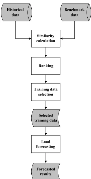
[image:2.595.342.503.45.359.2]The framework of the proposed model for short term load forecasting is shown in Figure 1. It consists of 7 steps listed below.
Fig. 1. The framework of the proposed load forecasting model
Step 1: All the historical load curves are collected as a time series.
Step 2: A given time interval before the target time is taken as the benchmark of training data.
Step 3: All continuous sub series of the same time interval are extracted as candidates of training data. Step 4: The distance from every sub series to the benchmark is calculated.
Step 5: The load curves are ranked based on the distances to the benchmark
Step 6: The top ranked load curves having the shortest distances to the benchmark are recognized as appropriate training data.
Step 7: A prediction model trained by the selected load curves is applied to forecast the load of the given day. As described before, a given time interval before the target time is taken as the benchmark of training data. The similarity between a load curve and the benchmark is measured by Euclidean distance shown as Equation (1).
∑
=−
=
ni
i
i
y
x
Y
X
d
1
2
)
(
)
,
(
(1)where X={x1, x2, …xn} and Y={y1, y2, …yn} are two nodes in
N - dimensional Euclidean space. The load curves of similar days with distances longer than a predefined threshold are removed from the training data.
III. PERFORMANCE EVALUATION
A. Data Preparation
January 2008 to December 2008 of a particular data set used. The dataset is downloaded from Duke Energy Carolinas (http://www.ferc.duke-energy.com/Load/Load.htm). The data of every day consists of 24 hour load information. The 12 months data is divided into two data sets. The first one, which contains 11 months data from January to November, is used for training. The other one containing the December data is used for testing.
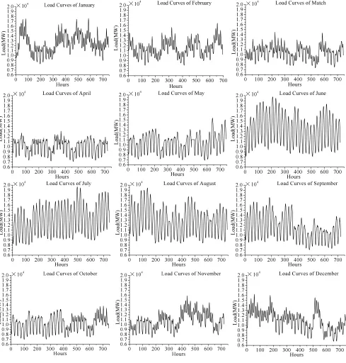
As described before, load curves have weekly and daily periodicity. The load curves of different months are shown in Fig. 2. As shown in Fig. 2, there is one peak or two in each day (24 hours) which represent the daily periodicity. Furthermore, the load of June, July and August are much higher than the load of other months due to the seasonal
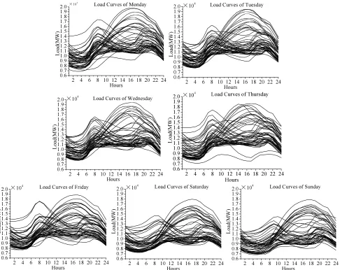
variation. Fig. 3 shows that the load curves of different day types (from Monday to Sundays) are relatively similar. Fig. 3 indicates that most load curves of the same day type have similar trend. As shown in Fig. 3, the load curves of the same load curves can be divided into two major types according to different seasons. The first type has two lower peaks and the second type has a higher peak. Most load curves have the same trends and similar values except a few abnormal ones, such as the lowest load curve in Fig. 3 (Thursday). Using abnormal data for training is likely to mislead the forecasting results. As revealed by the figures, the historical load curves with similar trends and values will be useful for load forecasting by filtering out the abnormal data, which is in accord with the motivation of this study.
0 100 200 300 400 500 600 700 0.6 0.7 0.8 0.9 1.0 1.1 1.2 1.3 1.4 1.5 1.6 1.7 1.8 1.9 2.0 L o ad (M W ) Hours
×104 Load Curves of January
0 100 200 300 400 500 600 700 0.6 0.7 0.8 0.9 1.0 1.1 1.2 1.3 1.4 1.5 1.6 1.7 1.8 1.9 2.0 L o ad (M W ) Hours
×104 Load Curves of February
0 100 200 300 400 500 600 700
0.6 0.7 0.8 0.9 1.0 1.1 1.2 1.3 1.4 1.5 1.6 1.7 1.8 1.9 2.0 L o ad (M W ) Hours
×104 Load Curves of Match
0 100 200 300 400 500 600 700
0.6 0.7 0.8 0.9 1.0 1.1 1.2 1.3 1.4 1.5 1.6 1.7 1.8 1.9 2.0 L oad( M W) Hours
×104 Load Curves of April
0 100 200 300 400 500 600 700
0.6 0.7 0.8 0.9 1.0 1.1 1.2 1.3 1.4 1.5 1.6 1.7 1.8 1.9 2.0 L o ad (M W ) Hours
×104 Load Curves of May
0 100 200 300 400 500 600 700
0.6 0.7 0.8 0.9 1.0 1.1 1.2 1.3 1.4 1.5 1.6 1.7 1.8 1.9 2.0 L oad( M W) Hours
×104 Load Curves of June
0 100 200 300 400 500 600 700 0.6 0.7 0.8 0.9 1.0 1.1 1.2 1.3 1.4 1.5 1.6 1.7 1.8 1.9 2.0 L o ad (M W ) Hours
×104 Load Curves of July
0 100 200 300 400 500 600 700
0.6 0.7 0.8 0.9 1.0 1.1 1.2 1.3 1.4 1.5 1.6 1.7 1.8 1.9 2.0 L o ad (M W ) Hours
×104 Load Curves of August
0 100 200 300 400 500 600 700
0.6 0.7 0.8 0.9 1.0 1.1 1.2 1.3 1.4 1.5 1.6 1.7 1.8 1.9 2.0 L o ad (M W ) Hours
×104 Load Curves of September
0 100 200 300 400 500 600 700
0.6 0.7 0.8 0.9 1.0 1.1 1.2 1.3 1.4 1.5 1.6 1.7 1.8 1.9 2.0 L oa d( M W ) Hours
×104 Load Curves of October
0 100 200 300 400 500 600 700
0.6 0.7 0.8 0.9 1.0 1.1 1.2 1.3 1.4 1.5 1.6 1.7 1.8 1.9 2.0 L oa d( M W ) Hours
×104 Load Curves of November
0 100 200 300 400 500 600 700
0.6 0.7 0.8 0.9 1.0 1.1 1.2 1.3 1.4 1.5 1.6 1.7 1.8 1.9 2.0 L o ad (M W ) Hours
[image:3.595.56.545.233.745.2]×104 Load Curves of December
2 4 6 8 10 12 14 16 18 20 22 24 0.6
0.7 0.8 0.9 1.0 1.1 1.2 1.3 1.4 1.5 1.6 1.7 1.8 1.9
2.0×10 Load Curves of Monday
4
Lo
ad
(MW)
Hours 2 4 6 8 10 12 14 16 18 20 22 24
0.6 0.7 0.8 0.9 1.0 1.1 1.2 1.3 1.4 1.5 1.6 1.7 1.8 1.9 2.0
L
o
a
d
(M
W
)
Hours
×104 Load Curves of Tuesday
2 4 6 8 10 12 14 16 18 20 22 24 0.6
0.7 0.8 0.9 1.0 1.1 1.2 1.3 1.4 1.5 1.6 1.7 1.8 1.9 2.0
L
o
ad
(M
W
)
Hours
×104 Load Curves of Wednesday
2 4 6 8 10 12 14 16 18 20 22 24 0.6
0.7 0.8 0.9 1.0 1.1 1.2 1.3 1.4 1.5 1.6 1.7 1.8 1.9 2.0
L
o
ad
(M
W)
Hours
×104 Load Curves of Thursday
2 4 6 8 10 12 14 16 18 20 22 24 0.6
0.7 0.8 0.9 1.0 1.1 1.2 1.3 1.4 1.5 1.6 1.7 1.8 1.9 2.0
L
o
ad
(M
W
)
Hours
×104 Load Curves of Friday
2 4 6 8 10 12 14 16 18 20 22 24 0.6
0.7 0.8 0.9 1.0 1.1 1.2 1.3 1.4 1.5 1.6 1.7 1.8 1.9 2.0
L
o
ad
(M
W
)
Hours
×104 Load Curves of Saturday
2 4 6 8 10 12 14 16 18 20 22 24
0.6 0.7 0.8 0.9 1.0 1.1 1.2 1.3 1.4 1.5 1.6 1.7 1.8 1.9 2.0
L
o
ad
(M
W
)
Hours
[image:4.595.58.544.50.436.2]×104 Load Curves of Sunday
Fig. 3. The load curves of different day types
B. Evaluation Metric and Baseline Methods
The forecasted result deviation from the actual values are evaluated in term of Mean Absolute Percentage Error (MAPE) shown in Equation (2).
∑
=
×
−
=
Ni
i A
i F i A
P
P
P
N
MAPE
1
100
|
|
1
(%)
(2)where PA, PFdenote the actual and forecasted values of the
load, respectively. N denotes the number of the hours of a
day in this work (N = 24).
An artificial neural networks (ANN) based method, which uses the load curves of the same hours for training, is taken as baseline method for comparison based on two reasons. The first reason is that ANN is proved to be efficient for load forecasting in literature, thus using ANN for comparison is fair enough. The second reason is that the improvement by using a novel training data selection strategy can be clearly revealed by using the same forecast model.
C. Results and Analysis
The forecasted results using the proposed approach compared with the actual load and the results of the
baseline method are shown in Fig. 4.
Fig. 4 vividly shows that the actual and forecasted load curves have similar trends and values. The performance of the proposed approach based on training data selection (TDS) is also measured in terms of the MAPE error. The performance is compared with the reference algorithm which is shown in Table I.
As shown in Table I, the proposed approach provides more than 1.01% higher performance on average
compared to the baseline method. These translate to
2 4 6 8 10 12 14 16 18 20 22 24 0.8
0.9 1.0 1.1 1.2 1.3 1.4 1.5 1.6
Hour
L
oad(
MW
)
Actual load Baseline Proposed method
×104 Load Curves of Dec 1
2 4 6 8 10 12 14 16 18 20 22 24 0.8
0.9 1.0 1.1 1.2 1.3 1.4 1.5 1.6
Hour
L
oad(
MW
)
Actual load Baseline Proposed method Load Curves of Dec 2
×104
2 4 6 8 10 12 14 16 18 20 22 24 0.9
1.0 1.1 1.2 1.3 1.4 1.5 1.6 1.7
Hour
L
oad(
MW
)
Actual load Baseline Proposed method
Load Curves of Dec 3
×104
2 4 6 8 10 12 14 16 18 20 22 24
0.8 0.9 1.0 1.1 1.2 1.3 1.4 1.5 1.6
Hour
L
o
ad
(M
W
)
Actual load Baseline Proposed method Load Curves of Dec 4 ×10⁴
2 4 6 8 10 12 14 16 18 20 22 24 0.8
0.9 1.0 1.1 1.2 1.3 1.4 1.5 1.6
Hour
L
oad(
MW
)
Actual load Baseline Proposed method Load Curves of Dec 5
×104
2 4 6 8 10 12 14 16 18 20 22 24 0.8
0.9 1.0 1.1 1.2 1.3 1.4 1.5 1.6
Hour
L
oad(
MW
)
Actual load Baseline Proposed method Load Curves of Dec 6
×104
2 4 6 8 10 12 14 16 18 20 22 24 0.8
0.9 1.0 1.1 1.2 1.3 1.4 1.5 1.6
Hour
L
oad(
MW
)
Actual load Baseline Proposed method
Load Curves of Dec 7
×104
Fig. 4. The actual and forecasted load curves
TABLEI
PERFORMANCE OF THE PROPOSED APPROACH AND THE BASELINE METHOD
MAPE(%) Day
Baseline Selected
Dec 1(Monday) 6.21 6.7 Dec 2(Tuesday) 5.18 3.19 Dec 3(Wednesday) 7.96 5.32 Dec 4(Thursday) 4 3.7 Dec 5(Friday) 4.16 3.61 Dec 6(Saturday) 2.79 2.92 Dec 7(Sunday) 5.10 2.89 Overall 5.06 4.05
IV. CONCLUSION
This paper presents a novel approach for short term load forecasting by selecting appropriate training data. Compared to the previous studies, the load curve of a time interval before the target hour is regard as the benchmark of training data instead of the cluster center of all historical data used in previous studies. Second, all the continuous sub series of the
same time interval are regard as candidates for training in the proposed method. Thus more appropriate training data can be extracted by using the proposed method. Experiments are conducted on the real load data to verify the efficiency of the proposed approach. The proposed approach outperforms the baseline method using the same prediction model. It achieves 20% improvements over the baseline method. The approach achieves promising results by using only historical load data which is shown in this study. The performance could be further improved by considering more factors such as weather changes.
REFERENCES
[1] A. D. Papalexopoulos and T. C. Hesterberg, “A regression-basedapproach to short-term load forecasting,” IEEE Trans. Power Syst., vol.5, no. 4, pp. 1535–1550, 1990.
[2] S. J. Huang and K. R. Shih, “Short-term load forecasting via ARMA model identification including nongaussian process considerations,”IEEE Trans. Power Syst., vol. 18, no. 2, pp. 673–679, 2003.
[4] H. S. Hippert, C. E. Pedreira, and R. C. Souza, “Neural networks for short-term load forecasting: A review and evaluation,” IEEE Trans.Power Syst., vol. 16, no. 1, pp. 44–55, 2001.
[5] Zhiyong Wang, Chuangxin Guo, Quanyuan Jiang and Yijia Cao. A Fault Diagnosis Method for Transformer Integrating Rough Set with Fuzzy Rules. Transactions of the Institute of Measurement and Control, Vol. 28, No. 3, 243-251 (2006)
[6] Al-Hamadi H, Soliman S. 2004. Short-term load forecasting based on Kalman filtering algorithm with moving window weather and load model. EPSR- Electric Power System Research. 68: 47-59.
[7] T. Haida and S. Muto, “Regression based peak load forecasting using a transformation technique,” IEEE Trans. Power Syst., vol. 9, no. 4, pp.1788–1794, 1994.
[8] S. Rahman and O. Hazim, “A generalized knowledge-based short term load-forecasting technique,” IEEE Trans. Power Syst., vol. 8, no. 2, pp.508–514, 1993.
[9] H.Wu and C. Lu, “A data mining approach for spatial modeling in small area load forecast,” IEEE Trans. Power Syst., vol. 17, no. 2, pp. 516–521, 2003.