Model Reduction for a Variable Geometry
Fluid Thermal Problem
Elliott Bach´e, Jose M. Vega, and A. Vel´azquez
Abstract—A methodology is presented to create reduced models of fluid thermal problems with varying geometry. The methodology is applied to the nonisothermal backward-facing step problem, depending on three parameters: the Reynolds number, the wall temperature, and the step height. Various snapshots are calculated using a computational fluid dynamics (CFD) solver in disparate grids, which are transformed into a generic grid by means of a smooth function. A proper orthogonal decomposition basis is created for these transformed snapshots, the flow variables are expanded into the resulting modes, and the reconstructed flow variable distributions are transformed back into the original grids. The associated mode amplitudes are calculated minimizing (using a genetic algo-rithm) a residual, which is defined using a limited number of grid points (which lessens the computational effort). The resulting reduced order model provides solutions that compare well with their CFD counterparts, in a much smaller CPU time.
Index Terms—Proper orthogonal decomposition, variable geometry, reduced order model.
I. INTRODUCTION
R
EDUCED order models (ROMs) are becoming more and more efficient and thus more appealing for indus-trial applications. Applications such as optimization and con-ceptual design can be easily handled with a ROM, reducing the time span from the beginning phase to the final phases of the design process. A review of advances in such ROMs is presented in [10].Although ROMs are becoming widespread in many types of applications, there are not that many that deal with varying geometries. The varying geometry involves difficulties for example when applying proper orthogonal decomposition (POD). In order to surmount these difficulties, a few tech-niques have been proposed account for varying geometries, such as those presented in [3], [15], [17], [13], [8], [12], and [14]. Among these, the authors employ such methods as a multi-POD approach (using a POD basis for each grid deformation) and mapping the grid displacement as a parameter. There are however no cases where they create a POD basis with varying grids.
In this paper, a POD-based ROM that takes into account a variable geometry as one of the parameters will be developed. The paper is a continuation of the related former work by us [1], [2], which presented the same type of ROM but with fixed geometries.
Manuscript received March 6th, 2011; revised March 29th, 2011. This research was supported by the Spanish Ministry of Education and Science (MEC) under Projects DPI2009-07591 and TRA2010-18054.
E. Bache and A. Velazquez are in the Aerospace Propulsion and Fluid Mechanics Department, School of Aeronautics, Universidad Politec-nica de Madrid, Plaza del Cardenal Cisneros 3, 28040 Madrid, Spain e-mail: [email protected] [email protected]
[image:1.595.303.552.164.245.2]J. M. Vega is in the Applied Mathematics Department, School of Aero-nautics, Universidad Politecnica de Madrid, Plaza del Cardenal Cisneros 3, 28040 Madrid, Spain. e-mail: [email protected]
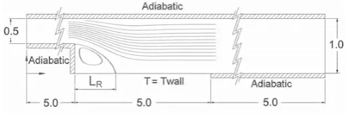
Fig. 1. Sketch of the test problem configuration. Flow goes from left to right.
II. APPLICATIONDESCRIPTION
A. Flow Description
The test problem to illustrate the methodology is a 2D laminar, incompressible flow through a backward-facing step with a portion of the lower wall being heated. In the equations and boundary conditions below, all distances were rendered dimensionless using the hydraulic diameter of the inlet channel (twice the inlet height). The velocity, pressure, and temperature are non-dimensonalized with the mean inlet velocity, the inlet dynamic pressure, and the inlet temperature, respectively.
The governing equations are
∂xu+∂yv= 0, (1)
u∂xu+v∂yu+∂xp−
µ∆u+ 2∂xµ∂xu(∂yu+∂xv)
Re = 0,
(2)
u∂xv+v∂yv+∂yp−
µ∆v+ 2∂xµ∂xv(∂xv+∂yu)
Re = 0, (3)
u∂xT+v∂yT−
κ∆T +∂xκ∂xT+∂yκ∂yT
ReP r = 0, (4)
where∂xand∂ystand for partial derivatives,∆ =∂xx2 +∂yy2 is the Laplacian operator, and the inlet Reynolds and Prandtl numbers are defined as
Re= 2 ˜ρinlet˜hinletu˜inlet/µ˜( ˜Tinlet), Pr= ˜cpµ˜( ˜Tinlet)/˜κ( ˜Tinlet).
(5)
Here,u˜inletis the mean inlet velocity and tildes denote di-mensional quantities.µandκare the dimensionless viscosity and thermal conductivity, which (in the considered tempera-ture range, assuming that the working fluid is water) depend on temperature asµ = 1−5.646(T−1) + 12.26(T −1)2
and κ= 1 + 0.786(T −1)−1.176(T −1)2, which result
from well known correlations [16].
free condition is imposed, namely ∂xu = ∂xv = ∂2xxp =
∂xT = 0. At the walls, we impose noslip (u=v= 0), and the following thermal conditionsT =Twallif5< x <10.5 andy= 0, andu=v = 0, ∂nT = 0. Here, n stands for the direction normal to the wall.
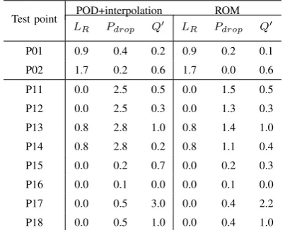
[image:2.595.47.288.258.330.2]The CFD computations needed to generate the snapshots are carried out with the solver described in [16]. Three free parameters are present, namely the Reynolds number, the wall temperature downstream of the step, and the step height. The maximum Reynolds number (400) is selected to preserve the hypothesis that the flow is two dimensional [16], [4], [7], and [5]. The step height is allowed to change in a rather wide range (0.1 to 0.6), which involves large changes in both the geometry and flow topologies. An idea of the severity of this change is provided in Fig. 2, where the streamlines patterns are shown for three representative cases. Solving the
Fig. 2. Streamlines for the cases:Re= 100, Tw= 1.0, H= 0.1(top),
Re= 200, Tw= 1.1, H= 0.4(middle), andRe= 400, Tw= 1.2, H=
0.6(bottom).
problem also requires drastic changes in the computational mesh, both in the number of points (which are 6,347, 12,485, and 16,577 in the three cases considered in Fig.2) and in their distribution (which involves drastic changes of mesh size, see Fig.3). Initially, snapshots are computed for the following 210 combinations of parameters:
• Re=100, 150, 200, 250, 300, 350, and 400, • Tw=1.0, 1.05, 1.10, 1.15, and 1.20,
• H =0.1, 0.2, 0.3. 0.4, 0.5, and 0.6.
Later on (see below), one additional series of snapshots will be computed in the case H = 0.15 to improve results, which will increase the total number of snapshots to 245. To assess the ROM accuracy, a series of 10 test points has been defined inside the parametric space, see Table I. Three figures of merit have been chosen to compare the ROM and CFD results, namely the reattachment length, LR, of the recirculation region located directly downstream of the step, the pressure drop,Pdrop, between entrance and exit, and the heat flux across the heated portion of the lower wall behind the step (see Fig.1). The latter is accounted for using the heat flux per unit width, defined as
Q′=∑∂yT(x,0)κ(T(x,0)) (6)
where Q′ is the dimensional heat flux across the non-adiabatic part of the lower wall. The actual CFD values of these figures of merit at the test points are given in Table I
III. METHODDESCRIPTION
A. Virtual grid
The mesh used in the CFD calculations is separated into 5 different zones, as plotted in Fig. 3-top. A close-up view
TABLE I
DEFINITION OF TEST POINTS ANDCFDVALUES OF THE FIGURES OF
MERIT
Problem parameters Figures of merit Test point
Re Twall H LR Pdrop Q˜′
P01 225 1.075 0.35 1.783 1.094 3.202
P02 275 1.125 0.45 2.917 0.727 5.347
P11 125 1.025 0.15 0.317 3.318 1.088
P12 125 1.175 0.15 0.383 3.026 8.702
P13 125 1.025 0.55 1.983 1.963 0.734
P14 125 1.175 0.55 2.167 1.910 5.980
P15 375 1.025 0.15 0.683 0.921 1.507
P16 375 1.175 0.15 0.817 0.836 12.21
P17 375 1.025 0.55 4.350 0.417 0.905
P18 375 1.175 0.55 4.400 0.420 7.748
of the near-corner CFD grid distribution is shown in Fig. 3-bottom. Varying geometries and mesh topologies cannot be
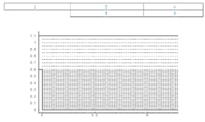
Fig. 3. Top: overview of a typical CFD domain with the different zones. Bottom: grid points distribution in the vicinity of the step for the case H= 0.5.
used in a standard POD, which requires a fixed geometry (with fixed mesh points). Thus, a virtual geometry is first defined as the case with a step size H = 0.3. In this, a virtual mesh is defined as the Cartesian equispaced mesh with five zones that are the counterparts of the zones in the CFD meshes. In both cases the x-y spacing between mesh points is as follows: zone 1: 0.1 x 0.05, zone 2: 0.01667 x 0.05, zone 3: 0.01667 x 0.01667, zone 4: 0.45 x 0.05, zone 5: 0.45 x 0.01667. Now, transformation between the virtual geometry and the actual geometries for each value of the step height H is done mapping the vertical coordinate, using the logarithmic function
η=Aln(By+ 1) (7)
where A and B are determined requiring thatη(H) = 0.3and
[image:2.595.322.528.322.444.2]B. POD + interpolation
N snapshots are computed with the CFD solver presented in [11] and must be representative of the parameter range we intend to cover, namely
(uk, vk, pk, Tk) for k= 1, ..., N. (8)
Each snapshot gives the steady state of the system for a specific set of values of the parameters. These snapshots are first projected into the virtual geometry using (7) and then used to obtain the POD modes, which are calculated independently for each variable. For instance, POD modes for the horizontal velocity are given by
Uj = N ∑
k=1
αkjuk, (9)
where the coefficients αkj are such that (α1
1, ..., αN1), ...,(αN1, ..., αNN) are the eigenvectors of the positive definite, symmetric N xN-matrix R, known as the covariance matrix, defined as
Rij =⟨ui, uj⟩ (10) where Ω is the following projection window in the virtual geometry.
Ω : 6< x <10, 0< y <0.8, (11)
Note that we are not taking the whole fluid domain to calculate POD modes, which would be quite computation-ally expensive. This simplification has been explained and checked in reference [2]. Now, if the expansion (9) is truncated ton≤Nterms, then the relative, root mean square (RMS) error is bounded by
|error| ≤ v u u t ∑N
i=n+1 γi
/∑N
i=1
γi (12)
where γ1 ≥ ... ≥ γN ≥ 0 are the eigenvalues of the covariance matrix (10). This gives an a priori estimate of the number of POD modes that must be retained to obtain a fixed error. After truncation and projection back into the CFD geometry, the POD modes are used to calculate the flow variables as
u(x, y) =
n1
∑
i=1
A1iUi(x, y) v(x, y) = n2
∑
i=1
A2iVi(x, y)
p(x, y) =
n3
∑
i=1
A3iPi(x, y) T(x, y) = n4
∑
i=1
A4iTi(x, y)
(13) where the POD-mode amplitudesA1
i, ..., A4i are unknowns to be determined below. As an initial guess for the optimization process below, we shall use a first approximation of the amplitudes for arbitrary parameter values using POD + interpolation [1]; see also [6], [9] for related combinations of POD like methods and interpolation. The amplitudes of the modes (in terms of these parameters) are calculated in two steps: (a) at the parameter values associated with the snap-shots, the POD-mode amplitudes Aji = Aji(Re, Twall, H) are obtained by just projecting the snapshots (8) into the POD basis, which requires projecting back and forth into the virtual mesh; and (b) at the remaining (intermediate) values of the parameters, each mode amplitude is calculated using
POD to obtain joint modes associated with dependence on the three parameters and cubic spline interpolation in each of these joint modes; see [1] for more details.
C. The overall residual
As anticipated above, the next step consists in calculating the POD-mode amplitudes (i.e. the coefficients in the expan-sions (13)) by minimizing the following residual (see [2])
Residual=∑4j=1N1
E|Ej(xk, yk)|
+∑4j=1N1
BC|BCj(xk, yk)|,
(14)
where (xk, yk) are all points in the following projection window
6< x <10 0< y <0.5 +H (15)
which is the counterpart of the projection window in the virtual geometry that was used above to calculate POD modes (cf eq.(11) and see Fig. 2);Ejare the left hand sides of eqs. (1)-(4) and
BC1=u(p, ymiddle)
−{−24(ymiddle−H) [
(ymiddle−H)−12 ]}
,
(16)
BC2= ∂p ∂x−
(
− 48
Re
)
≈ ∆pin
∆xin−
(−48
Re), (17)
BC3=T(0, ymiddle)−Tentrance, (18)
TABLE II
RELATIVE ERRORS IN%RESULTING FROM BOTHPOD+INTERPOLATION
ANDROMCALCULATIONS ON THE FIGURES OF MERIT,USING210
SNAPSHOTS AND RETAINING15MODES. PODMODES ARE CALCULATED
IN THE PROJECTION WINDOW(11)AND THE RESIDUAL IS CALCULATED
FROM50EQUISPACED POINTS IN THE PROJECTION WINDOW(15).
POD+interpolation ROM Test point
LR Pdrop Q′ LR Pdrop Q′
P01 0.0 0.5 0.4 1.9 0.4 0.1
P02 1.1 0.2 2.1 1.1 0.1 2.2
P11 10.5 3.6 0.0 10.5 2.5 4.0
P12 8.7 3.4 0.5 13.0 2.4 0.4
P13 0.8 2.8 0.5 0.0 1.0 1.0
P14 0.8 2.8 0.1 0.8 7.1 0.2
P15 14.6 1.8 1.3 17.1 1.4 1.3
P16 14.3 1.7 1.2 14.3 0.9 1.0
P17 1.5 0.5 6.7 1.9 0.5 8.4
P18 0.4 0.5 2.2 0.4 0.3 2.0
IV. RESULTS
[image:4.595.324.526.415.578.2]To begin with, the ROM developed above is applied retain-ing the 15 most energetic POD modes calculated from the above defined 210 snapshots, using the projection window (11); the residual is calculated using only 50 equispaced points in the projection window (15). Relative errors (in %) on the three figures of merit at the test points are qiven in Table II as calculated using both POD+interpolation and the ROM; see Table I for the definition of the test points and the CFD calculated values of the figures of merit. Note that both POD+interpolation and ROM errors are always smaller than 4%, except for the reattachment length at test points P11, P12, P15, and P16 and the heat flux at test point P17. The reason for this lower accuracy seems to be due to the fact that POD approximations tend to deteriorate when either:
a) The step height is small (test points P11, P12, P15, and P16, see Table 1) because flow structures have a much smaller size than for larger values of H.
b) Or the wall temperature is lowest (test point P17), because heat transfer in this case is associated with small values of the heat flux near the walls.
In both cases, the actual numerical resolution in POD might be not sufficient. In order to deal with this difficulty, two improvements have been made in the method:
1) Increasing the number of snapshots with 35 additional ones at a step height H = 0.15. Results are given in Table III and show that results improve everywhere. Also, errors are now smaller than 2.4 % (including the approximation ofLR at P15 and P16), except for the reattachment length at P11 and P12 and the heat flux at P17, which are exact only within 8.7%. In any event, deviations of this order are admissible from the point of view of, for example, micro-electro-mechanical sys-tems (MEMS) design engineering applications since, in this context, experimental work has uncertainties of the order of±10%.
2) Using the same 245 snapshots as in case (a), but retaining twice the number of modes (a total of 30, instead of 15). The results obtained are presented in
TABLE III
SAME ASTABLEII,BUT USING245SNAPSHOTS
POD+interpolation ROM Test point
LR Pdrop Q′ LR Pdrop Q′
P01 0.9 0.4 1.4 0.0 0.1 2.0
P02 1.1 0.2 2.4 1.1 0.2 2.5
P11 5.2 2.6 0.7 5.2 1.7 0.3
P12 4.4 2.5 0.1 8.7 1.2 0.2
P13 0.8 2.8 0.2 1.7 0.9 0.5
P14 0.8 2.8 0.1 0.8 0.6 0.3
P15 0.0 0.3 1.3 0.0 0.1 1.3
P16 2.0 0.4 0.8 2.0 4.0 5.4
P17 1.5 0.5 6.9 1.9 1.2 7.5
P18 0.4 0.5 2.4 0.4 0.2 2.1
Table IV, and show that now accuracy is quite good for the three figures of merit in the ten test points. Also, results obtained using the ROM (within 1.5% accuracy) are consistently better than those obtained using POD+interpolation (2.8% errors). It is to be noted, however, that this improvement came at the expense of a larger computational time. While each run of the ROM in Table III is performed in only 3-7 CPU minutes, each run in Table IV requires 10-30 minutes.
TABLE IV
SAME ASTABLEII,BUT USING245SNAPSHOTS AND30MODES
POD+interpolation ROM Test point
LR Pdrop Q′ LR Pdrop Q′
P01 0.9 0.4 0.2 0.9 0.2 0.1
P02 1.7 0.2 0.6 1.7 0.0 0.6
P11 0.0 2.5 0.5 0.0 1.5 0.5
P12 0.0 2.5 0.3 0.0 1.3 0.3
P13 0.8 2.8 1.0 0.8 1.4 1.0
P14 0.8 2.8 0.2 0.8 1.1 0.4
P15 0.0 0.2 0.7 0.0 0.2 0.3
P16 0.0 0.1 0.0 0.0 0.1 0.0
P17 0.0 0.5 3.0 0.0 0.4 2.2
P18 0.0 0.5 1.0 0.0 0.4 1.0
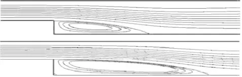
Fig. 4. Comparison between CFD (solid) and ROM (dashed) streamlines at test points P01 (top) and P17 (bottom)
Fig. 5. Comparison between CFD (solid) and ROM (dashed) isobars at test points P01 (top) and P17 (bottom)
the main recirculation bubble is always well approximated even though the projection window excluded also the main recirculation bubble in some cases (Fig. 2-up) and a large part of this bubble in some other cases (Fig. 2-middle). All these illustrate both (a) the power of POD when this method is properly used and (b) the fact that the ROM is quite robust in the sense that selection of the projection window is not critical. Now, a question arises on whether the results above can be improved with a better selection of both the projection window and the points where the residual are calculated. Concerning the latter, note that choosing 50 equispaced points in the projection window (15), as we did in Tables II-IV to calculate the residual means that, for instance, that zone affected by the first recirculation bubble (0< y < H) contains 18 points whenH = 0.1and 40 points when H = 0.6. This suggests two improvements:
• A first improvement results from maintaining the projec-tion windows (15) and (11), but increasing the number of points in the residual calculation to 100, and ensuring that 70 of them are in that part of the projection window affected by the first recirculation bubble (0< y < H). Results are shown in Table 5-left. Comparison with Table IV shows that a significant improvement results from the increase in the number of points and the better selection of the 100 points. Note that errors are within 2.3% except for the reattachment length at point P11 and the heat flux at point P17; but note that the CFD values of and heat flux at these points are quite small, which explains the larger relative errors.
• The projection window can be split into two sub-windows in such a way that they roughly cover those regions affected by the recirculation bubbles. Namely,
6< x <10,0< η <0.3; 9< x <13,0.3< η <0.8 (20) 6< x <10,0< y < H; 9< x <13,0.5< y < H
(21)
Fig. 6. Comparison between CFD (solid) and ROM (dashed) isotherms at test points P01 (top) and P17 (bottom)
in the virtual and CFD geometries, respectively. Also, the residual is calculated taking 50 and 15 points in the first (6 < x < 10) and second (9 < x < 13) sub-windows, respectively. Results are shown in Table 5-right and are quite similar to those resulting from the first improvement above, which shows that the whole process is quite robust.
TABLE V
TABLE5 RELATIVE ERRORS%ON THE FIGURES OF MERIT CALCULATED
WITH THEROMDESCRIBED INTABLEIII,BUT(LEFT)USING70+30
POINTS IN THE PROJECTION WINDOW(15),AND(RIGHT)USING TWO
PROJECTION SUB-WINDOWS,SEE(11)-(21).
One window, 70+30 points Two windows, 50+15 points Test point
LR Pdrop Q˜′ LR Pdrop Q˜′
P01 0.9 0.2 0.9 0.9 0.2 0.6
P02 1.7 0.1 2.3 1.7 0.1 2.4
P11 5.2 1.9 0.2 5.2 1.7 0.5
P12 0.0 1.3 1.5 0.0 1.3 0.7
P13 0.8 0.9 0.1 1.7 0.9 0.0
P14 0.8 0.6 0.3 0.8 0.6 0.3
P15 0.0 0.1 1.2 2.4 0.2 1.1
P16 2.0 1.0 2.7 0.0 0.3 0.8
P17 1.1 0.5 7.6 1.1 0.5 7.6
P18 0.4 0.1 2.2 0.4 1.6 2.2
V. CONCLUSIONS
A method has been presented to generate ROMs in fluid-thermal problems with variable geometry. In particular, the required CFD-calculated snapshots are obtained in compu-tational domains with variable shape and number of grid points. The results obtained show that the method is flex-ible, robust, and accurate enough to be used for practical engineering applications. In particular, three parameters are considered in the test problem, namely the Reynolds number, the wall temperature, and the step height, which could be considered as representative of a variety of industrial problems in which flow topology, thermal, and geometry properties need to be analyzed simultaneously. Some remarks about the results are now in order:
[image:5.595.53.289.192.274.2] [image:5.595.303.552.342.536.2]simplest projection window). The spatial distribution of the flow variables is also close enough to the CFD solution to be used for detailed analysis purposes. The CPU time needed to generate each of these ROM results is of the order of 3 minutes, which is much smaller that the time needed to generate a CFD solution (of the order of 8 to 10 hours).
2) The accuracy of the method degrades, as it could be expected when the selected test points are close to the boundary of the 3-D parametric space. In this case, discrepancies with the CFD solutions using the simplest ROM configuration (Table II) are of the order of 3% except at some points where they can be as large as 17%. The time needed to generate the ROM model goes up to about 7 minutes. Adding some snapshots in the region of lower step height (Table III) reduces the largest errors to 8.7%, which it is already acceptable for engineering purposes and still requires a CPU time of 7 minutes, which is quite competitive when compared to the time needed to generate a full CFD solution. 3) Accuracy can be increased either retaining more POD
modes (30 instead of 15, see Table IV), which gives excellent accuracy but requires a CPU time of 10-30 minutes (still competitive compared to CFD) or selecting better both the projection window and the points where the residual is calculated (Table V). This gives both an excellent precision (errors within 3% except at those points where the approximated quantities are really small, where it is still reasonable, of the order of 7%) and a fairly small CPU time (3-7 minutes). Concerning the latter improvement, it is convenient that the projection window includes at least a part of the structured flow regions (e.g., second recirculation bubble), and that the selected points to calculate the residual are located in a balanced way, namely that there is a sufficient amount of them in the most structured regions. Nevertheless, the method is robust enough in connection with all these guidelines since, for instance reasonable results (even in the second recirculation bubble) are obtained selecting a projection window that does not contain the second recirculation bubble (or even does not contain the first recirculation bubble either, see Fig. 2), and calculating the residual using equispaced points in the first projec-tion window, which puts only a few points in the first recirculation bubble.
4) For simplicity, we have retained the same number of POD modes in each flow variable, but this can of course be improved selecting an appropriate number of modes for each flow variable. This could be done in an efficient way using the a priori error estimate (12), which is based on the singular values of each POD.
5) Adding 15 additional snapshots in that region of the parameter space where the ROM results exhibited largest errors highly improves the efficiency at a rea-sonable computational cost. This opens the possibility of designing a method to select the snapshots in such a way that only a few of them are enough, if properly selected. Its number should be just somewhat larger than the number of POD modes (say, twice the number
of modes). The method would provide a dramatic reduction in computational time since it is essentially associated with the CFD calculations of the snapshots. The remaining calculations in the method are quite inexpensive after the improvements introduced above. 6) Gradient like methods could be used to dramatically decrease computational time, which as explained above would require a redefinition of the residual and an efficient calculation of the gradient. Some care should also be taken with non-uniqueness of local minima of the residual, which is under research.
ACKNOWLEDGMENT
The authors are in debt with Diego Alonso Fern´andez and Luis S. Lorente for their help with theory and verification of results.
REFERENCES
[1] D. ALONSO, A. VELAZQUEZ,ANDJ. VEGA,Robust reduced order modeling of heat transfer in a back step flow, Int. J. Heat Mass Tran., 52 (2008), pp. 1149–1157.
[2] ,A method to generate computationally efficient reduced order models, Comput. Method. Appl. M., 198 (2009), pp. 2683–2691. [3] J. S. R. ANTTONEN, P. I. KING, AND P. S. BERAN, Pod-based
reduced-order models with deforming grids, Math. Comp. Model., 38 (2003), pp. 41–62.
[4] B. F. ARMALY, F. DURST, J. C. F. PEREIRA,ANDB. SCHONUNG¨ ,
Experimental and theoretical investigation of backward-facing step flow, J. Fluid Mech., 127 (1983), pp. 473–496.
[5] D. BARKLEY, M. GOMES,ANDR. HENDERSON,Three dimensional instability in flow over a backward facing step, J. Fluid Mech., 473 (2002), pp. 167–190.
[6] T. BUI-THANH,Proper Orthogonal Decomposition Extensions and their Applications in Steady Aerodynamics, Master Thesis. Singapore-MIT Alliance, 2003.
[7] F. DURST ANDJ. C. F. PEREIRA,Time-dependent laminar backward-facing step flow in a two dimensional duct,, J. Fluid. Eng., 110 (1988), pp. 289–296.
[8] J. HOLLKAMP ANDR. GORDON,Reduced-order models for nonlinear response prediction: Implicit condensation and expansion, J. Sound Vib., 318 (2008), pp. 1139–1153.
[9] L. LORENTE, J. VEGA,ANDA. VELAZQUEZ, Generation of aero-dynamic databases using high order singular value decomposition, J. Aircraft, 25 (2008), pp. 1779–1788.
[10] D. LUCIA, P. BERAN,ANDW. SILVA,Reduced-order modeling: new approaches for computational physics, Prog. Aerosp. Sci., 40 (2004), pp. 51–117.
[11] B. MENDEZ AND A. VELAZQUEZ, Finite point solver for the simulation of a 2-d laminar incompressible unsteady flows, Com-put. Method. Appl. M., 193 (2004), pp. 825–848.
[12] M. P. MIGNOLET AND C. SOIZE, Stochastic reduced-order mod-els for uncertain geometrically nonlinear dynamical systems, Com-put. Method. Appl. M., 197 (2008), pp. 3951–3963.
[13] S. NIROOMANDI, I. ALFARO, E. CUETO,ANDF. CHINESTA, Real-time deformable models of non-linear tissues by model reduction techniques, Comp. Meth. Prog. BioMed., 91 (2008), pp. 223–231. [14] Y. ROUIZI, Y. FAVENNEC, J. VENTURA,ANDD. PETIT,Numerical
model reduction of 2d steady incompressible laminar flows: Applica-tion on the flow over a backward-facing step, J. Comput. Phys., 228 (2009), pp. 2239–2255.
[15] W. A. SILVA ANDR. E. BARTELS, Development of reduced-order models for aeroelastic analysis and flutter prediction using the cfl3d v6.0 code, J. Fluid. Struct., 19 (2004), pp. 729–745.
[16] A. VELAZQUEZ, J. ARIAS,ANDB. MENDEZ,Laminar heat transfer enhacement downstream of a backward facing step by using a pulsat-ing flow, Int. J. Heat Mass Tran., 51 (2008), pp. 2075–2089. [17] J. VIERENDEELS, L. LANOYE, J. DEGROOTE,ANDP. VERDONCK,