Powered Outer Probabilistic Clustering
Peter Taraba
Abstract—Clustering is one of the most important concepts for unsupervised learning in machine learning. While there are numerous clustering algorithms already, many, including the popular one — k-means algorithm, require the number of clusters to be specified in advance, a huge drawback. Some studies use the silhouette coefficient to determine the optimal number of clusters. In this study, we introduce a novel algorithm called Powered Outer Probabilistic Clustering, show how it works through back-propagation (starting with many clusters and ending with an optimal number of clusters), and show that the algorithm converges to the expected (optimal) number of clusters on theoretical examples.
Index Terms—clustering, probabilities, optimal number of clusters, binary valued features, emails.
I. INTRODUCTION
For over half a century, clustering algorithms have gener-ated massive research interest due to the number of problems they can cover and solve. As an example one can mention [1], where the authors use clustering to group planets, animals, etc. The main reason for the popularity of clustering algo-rithms is that they belong to unsupervised learning and hence do not require manual data labeling, in contrast to supervised learning, which can require the cooperation of many people who often disagree on labels. As an example one can even mention Pluto, the celestial body no longer considered a planet as of 2006. The advantage of using unsupervised over supervised learning is that rather than relying on human understanding and labeling, clustering algorithms rely purely on objective properties of the entities in question. A good clustering algorithm survey can be found in [2].
The largest obstacle for clustering algorithms is finding the optimal number of clusters. Some results on this topic can be found in [3], where the authors compare several algorithms on two to five distinct, non-overlapping clusters. As another example, one can mention [4], where the authors use a silhouette coefficient (c.f. [5]) to determine the optimal number of clusters.
In this study, we construct two theoretical datasets: one with clusters that are clearly defined and a second with clusters that have randomly generated mistakes. We then show that the algorithm introduced in this paper converges to the expected number of clusters for both the perfect and the slightly imperfect cluster examples.
This paper is organized as follows. In section 2, we describe the POPC algorithm. In section 3, we confirm on three theoretical examples that the algorithm converges to the expected number of clusters. In section 4, we present an additional example of real email dataset clustering. In section 5, we draw conclusions.
Manuscript received May 18, 2017; revised June 07, 2017.
P. Taraba is currently not affiliated with any institution, residing in San Jose, CA 95129. (phone: +1-650-919-3827; e-mail: [email protected]).
II. ALGORITHMDESCRIPTION
The Powered Outer Probabilistic Clustering (POPC) al-gorithm relies on computing discounted probabilities of dif-ferent features belonging to difdif-ferent clusters. In this paper, we use only features that have binary values0and1, which means the feature is either active or not. One can write the probability of featurefi belonging to clusterk as
p(cl(fi) =k) =
c(sj(fi) = 1, cl(sj) =k)Cm+ 1
c(fi = 1)Cm+N
,
wherec is the count function, clis the clustering classifica-tion,N is the the number of clusters, k∈ {1, . . . , N}is the cluster number,sj are samples in the dataset,sj(fi)∈ {0,1} is the value of feature fi for sample sj, and Cm is a multiplying constant (we use Cm = 1000 in this study). If we sum over all clusters for one feature, we get:
N X
k=1
p(cl(fi) =k) = 1,
and subsequently further over all featuresfi we get:
F X
i=1
N X
k=1
p(cl(fi) =k) =F. (1)
If we used (1) as the evaluation function, we would not be able to optimize anything, because the function’s value is constant no matter how we cluster our samples sj. Hence, instead of summing over probabilities, our evaluation func-tionJ uses higher powers of feature probabilities as follows:
J=
F X
i=1
J(fi) = F X
i=1
N X
k=1
pP(cl(fi) =k)≤F, (2)
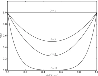
where P is the chosen power and we choose P > 1 in order to have a non-constant evaluation function. The main reason why this is desired can be explained with reference to a hypothetical case where there is only one feature and two clusters. We want samples with sj(f1) = 1 to belong
only to one of two clusters. In the case that samples are perfectly separated into the two clusters on the basis of the one feature, we maximizePN
k=1p
P(cl(f
i) =k)(value very close to 1 as we use discounting). In the case that some samples belong to one cluster and some to the other, so the separation is imperfect, we get a lower evaluation score (value significantly lower than1) for the feature. The higher the powerP, the lower the score we obtain when one feature is active in multiple clusters. This is displayed in Figure 1 for different powers P ∈ {1,2,3,10} and two clusters. For results reported in this paper we useP = 10.
0.0 0.2 0.4 0.6 0.8 1.0 p(cl(fi) = 1)
0.0 0.2 0.4 0.6 0.8 1.0
J(
fi
)
P = 1
P = 2
P = 3
[image:2.595.317.523.65.395.2]P = 10
Fig. 1. Values of the evaluation function for a hypothetical case where there is one feature and two clusters. If the feature is distributed between two different clusters, the evaluation functionJhas a lower value (near 0.5 on the x-axis). In case the feature belongs to only one cluster, or mostly to one cluster,J has a higher value for evaluation function (left near 0.0 or right near 1.0 on the x-axis — values close to optimumJ(fi) = 1).
increases as a result of reshuffling, the new cluster assign-ment is preserved. The algorithm ends when reshuffling no longer increases the evaluation function J.
The algorithm can be summarized in the following steps: 1) Using k-means clustering, assign each samplesj clus-tercl(sj) =k, where k ∈ {1, . . . , N} andN — the number of clusters — is chosen to be half the number of data samples.
2) Compute Jr=0 for the initial clustering, where r
de-notes the iteration of the algorithm.
3) Increase rtor:=r+ 1, start withJr=Jr−1.
4) For each samplesj, try to assign it into all the clusters to which it does not belong to (cl(sj)6=k)
a) If the temporary evaluation score JT with the temporarily assigned cluster improves over the previous value, i.e. JT > Jr, then assign Jr :=
JT and move samplesj to the new cluster. 5) IfJris equal toJr−1, then stop the algorithm.
Other-wise go back to step 3.
Remark (Implementation detail). The algorithm can be made faster if one saves the counts of different features for different clusters and updates these counts only if and when the evaluation score improves. This is just an implementation detail, which speeds up computations significantly and does not influence the result.
III. EXAMPLES
In this section, we create three theoretical examples, one perfect, one slightly imperfect and one with majority of noisy features.
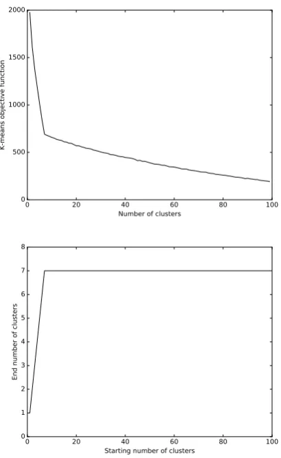
For the perfect example, we create a dataset containing 200 samples with100 features and assign each sample to a random cluster (N= 7) with a uniform discrete distribution, so that every cluster has approximately the same number of samples. In the same way, we assign every feature to a cluster. A feature is active (its value is1) only if the feature belongs to the same cluster as the sample and only eighty percent of the time.
0 20 40 60 80 100
Number of clusters 0
500 1000 1500 2000
K-m
ea
ns
ob
jec
tiv
e f
un
cti
on
0 20 40 60 80 100
Starting number of clusters 0
1 2 3 4 5 6 7 8
En
d n
um
be
r o
f c
lust
[image:2.595.68.264.68.220.2]ers
Fig. 2. (Top) K-means evaluation function depending on the number of clusters for example 1. (Bottom) Number of clusters created by the POPC algorithm depending on the number of starting clusters
Fig. 3. Theoretical example 1 - seven perfect clusters clustered by POPC. On vertical axis we have different samples belonging to different clusters (colors) and on horizontal axis we have different features.
In Figure 2 top, we show the k-means evaluation function depending on the number of clusters. There is a break-point at exactlyN = 7, the expected number of clusters. Figure 2 bottom shows the number of clusters created by the POPC algorithm. We can see that if we start with a number of clusters larger or equal to 7, we always end with the expected number of clusters 7.
First example clustered with POPC algorithm is displayed in Figure 3. As shown, clusters are found as expected.
[image:2.595.308.548.450.580.2]0 20 40 60 80 100 Number of clusters
0 500 1000 1500
K-m
ea
ns
ob
jec
tiv
e f
un
cti
on
0 20 40 60 80 100
Starting number of clusters 0
1 2 3 4 5 6 7 8
En
d n
um
be
r o
f c
lust
[image:3.595.63.268.63.397.2]ers
[image:3.595.311.514.72.184.2]Fig. 4. (Top) K-means evaluation function depending on the number of clusters for example 2. (Bottom) Number of clusters created by the POPC algorithm depending on the number of starting clusters.
Fig. 5. Theoretical example 2 - seven imperfect clusters clustered by POPC. On vertical axis we have different samples belonging to different clusters (colors) and on horizontal axis we have different features. Last ten percent features (on right) are the features, which do not belong to any cluster and are active twenty percent of time.
active twenty percent of time. The results for example 2 are displayed in Figure 4. The POPC algorithm introduced in this paper once again yields the expected number of clusters.
Second example clustered with POPC algorithm is dis-played in Figure 5. As shown, clusters are found as expected despite having small amount of imperfect features.
For theoretical example 3, we create 7 clusters with every cluster having 30 samples with 20 features. Every cluster has exactly one feature, which is active only for the cluster it belongs to. Remaining 13 features are random features, which do not belong to any cluster and are activate fifty
[image:3.595.313.512.246.358.2]per-Fig. 6. Theoretical example 3 - seven imperfect clusters clustered by k-means. On vertical axis we have different samples belonging to different clusters (colors) and on horizontal axis we have different features.
Fig. 7. Theoretical example 3 - seven imperfect clusters clustered by POPC. On vertical axis we have different samples belonging to different clusters (colors) and on horizontal axis we have different features. First 7 features (from left) are the significant features of respective clusters. Remaining 13 features are non-significant features, which do not belong to any cluster and are active fifty percent of time.
cent of time. This is main example, which shows why POPC algorithm is so useful. K-means algorithm due to majority of features being randomly active cannot find features which are significant features for clusters and finds clusters which are not the way we would expect them. Evaluation function
Jk−meansis very close to 0 even if we knew we are looking
for 7 clusters. This is displayed in Figure 6.
On other hand, when we use POPC algorithm we find exactly 7 clusters we expected and more importantlyJP OP C is close to 7, which is amount of features that are significant to respective clusters. This is displayed in Figure 7. This last theoretical example explains why in real life situations, POPC is not only able to find correct number of clusters, but also to find significantly better clusters than k-means for binary feature datasets.
All the theoretical examples introduced in this paper can be generated with C# code which can be downloaded from [6]. Same code contains implementation of popc algorithm.
IV. REAL LIFE EXAMPLE-EMAIL DATASET
[image:3.595.51.287.449.580.2]0 20 40 60 80 100 120 140 Number of clusters
0 100 200 300 400 500 600 700
K-m
ea
ns
ob
jec
tiv
e f
un
cti
on
0 20 40 60 80 100 120
Starting number of clusters 0
5 10 15 20 25
En
d n
um
be
r o
f c
lust
[image:4.595.328.523.53.257.2]ers
Fig. 8. (Top) K-means evaluation function depending on the number of clusters for real life example (emails). (Bottom) Number of clusters created by the POPC algorithm depending on the number of starting clusters
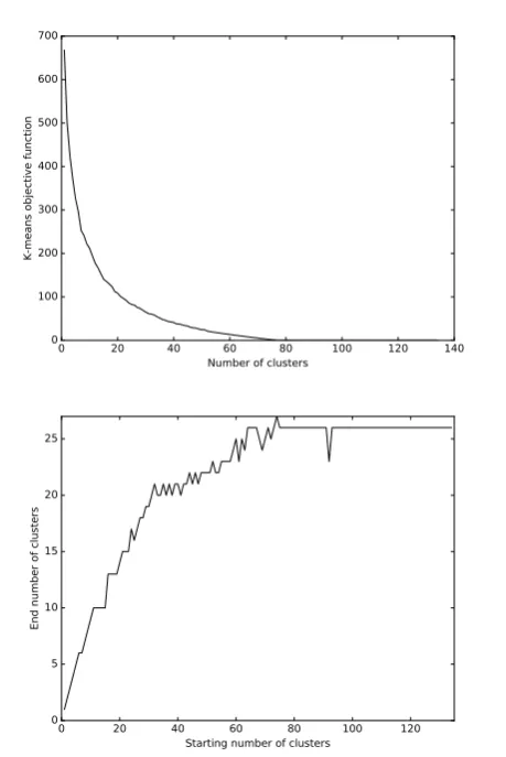
algorithm introduced in this paper settles on a final clustering with26clusters.
The email dataset contains 270 emails (samples) and 66 people (features). The final score for the evaluation func-tion with 26 clusters is J = 52.19 out of the maximum possible value 66. Even if we knew the correct number of clusters (which we do not) and used it with k-means, the evaluation function introduced in this paper would be
Jk−means= 32.91, which is significantly lower than52.19.
This represents an improvement in cluster quality of 29.21 percent. The score reflects approximately the number of people who belong only to a single cluster. Email clusters for the email dataset are displayed in Figure 9. Improvement over k-means was confirmed on emails of two other email datasets belonging to other people. Due to privacy issues, email dataset is not shared as it belongs to a private company.
[image:4.595.55.285.54.398.2]Remark(Interesting detail). While the maximum evaluation function value can be achieved by assigning all samples to the same single cluster, when starting with a large number of clusters, the algorithm does not converge even for real life datasets to a single cluster due to the use of back-propagation and the presence of local maximums along the way which result from reshuffling only a single sample at a time. This provides unexpected, but desired functionality. For the same reason, we are not able to start the algorithm with one cluster and subsequently subdivide the clusters, because
Fig. 9. Email clustering example. Emails are displayed as ’o’ in different cluster circles, people are displayed as ’+’ and connections between emails and people included on these emails are displayed as blue lines in between them.
this would only lower the evaluation function’s value. Hence, the algorithm works only backwards.
V. CONCLUSIONS
We introduced a novel clustering algorithm POPC, which uses powered outer probabilities and works backwards from a large number of clusters to the optimal number of clusters. On three theoretical examples, we show that POPC converges to the expected number of clusters. In a real life example with email data, we show that it would be difficult to determine the optimal number of clusters based on the k-means evaluation score, but when the algorithm introduced in this paper is used, it settles on the same number of clusters if we start with a large enough initial number of clusters. Importantly, the clusters are of higher quality in comparison with those produced by k-means even if we happened to know the correct number of clusters ex ante. Software Small Bang, which clusters emails and uses POPC algorithm can be downloaded from [7].
ACKNOWLEDGMENT
The authors would like to thank David James Brunner for many fruitful discussions on knowledge workers information overload as well as proofreading of the first draft. The authors would also like to thank anonymous reviewers for providing feedback which led to significant improvement of this paper.
REFERENCES
[1] J. Hartigan,Clustering Algorithms. John Wiley & Sons, 1975. [2] R. Xu and D. Wunsch, “Survey of clustering algorithms,”IEEE
Trans-actions on Neural Networks, vol. 16, 2005.
[3] G. Milligan and M. Cooper, “An examination of procedures for deter-mining the number of clusters in a data set,”Psychometrika, vol. 50, 1985.
[4] G. Frahling and C. Sohler, “A fast k-means implementation using coresets,”Int. J. Comput. Geom. Appl., vol. 18, 2008.