Change and invariance in EU aggregate financial statement data

CHANGE AND INVARIANCE IN EU AGGREGATE FINANCIAL STATEMENT DATA

By

C. Serrano Cinca

Department of Accounting and Finance

University of Zaragoza, Spain.

[email protected]

C. Mar Molinero

Department of Management

University of Southampton, UK.

[email protected]

J.L. Gallizo Larraz

Department of Accounting and Finance

University of Zaragoza, Spain.

[email protected]

This version: August 2001

The work reported in this paper was supported by grant 2FD97-2091 of the European Regional Development Fund (ERDF) under the title “Financial analysis of diversification and similarity of productive structures in the European Union”, administered by the University of Zaragoza, Spain.

CHANGE AND INVARIANCE IN EU AGGREGATE FINANCIAL STATEMENT DATA

ABSTRACT

Aggregate accounting data from the BACH data base for European manufacturing companies is used to explore the nature of the differences in financial structure between eleven countries in the European Union over the period 1986-1999. The analysis relies on scaling methods, which visualise the most important features of the data and their dynamic evolution. It is found that there is a geographical divide in the EU, which appears to be related to company profitability and staff cost structure. The differences between countries are influenced by the economic cycle, being more accentuated in periods of low economic activity.

1. INTRODUCTION

Is there a North-South divide in European Business? If there is such a divide, does it find its way to company financial statements? How can it be revealed using statistical tools? How does it evolve? What remains constant over time? How is it influenced by the economic cycle? These are the questions that guide the research summarised in this paper.

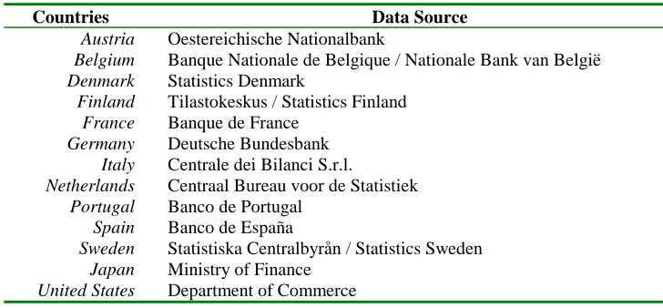
Since the 1980’s company financial statements have been collected and aggregated by Central Banks or other central statistical institutions. These statements are harmonised by the Directorate-General for Economic and Financial Affairs of the European Commission, and collected in the BACH (Bank for the Accounts of Companies Harmonised) database, European Commission (2000), ECCBSO (1995). A list of the institutions that contribute data to BACH can be found in Table 1. The European Commission publishes transition tables to convert national accounts into BACH conventions, European Commission (2000). This data set presents a unique opportunity to conduct comparative accounting studies in European Business and its evolution over time. Such studies are rare with European data, although they have been made using North American company accounts, Braun and Traichal (1999).

*************** Table 1 about here. ***************

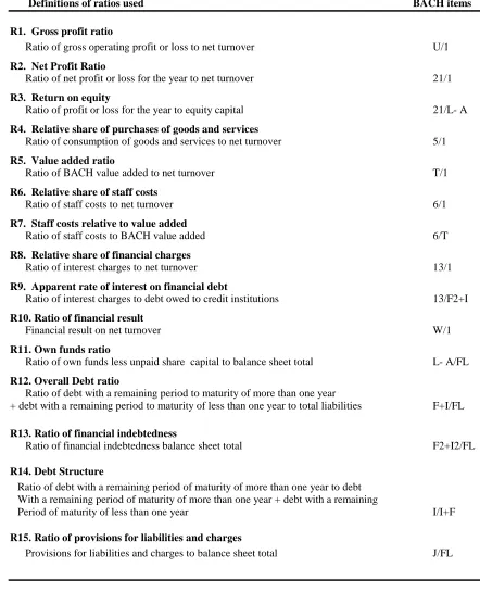
and Fieldsend (1987), but no further mention will be made of this aspect in this paper. The list of ratios and their definitions can be seen in Table 2.

*************** Table 2 about here. ***************

It could be conjectured that if there are differences between companies in the various countries, these will be reflected in the BACH ratio structure. It can be further presumed that if these structures evolve differently over time, perhaps as a result of different reactions to the economic cycle, it will also be possible to analyse them by studying the dynamic behaviour of these ratios.

The data set is three-way: ratios by country and by year. Many statistical tools are available to study three way data, such as, for example, panel data methods, Markus (1979), or dynamic factor analysis, which is particularly appropriate for time series data, Geweke (1977). However, we prefer to use scaling methods, which have strong statistical foundations, but visualise the main characteristics of the data. Many scaling approaches exist to study three way data such as, for example, Tucker (1966), Harshman (1970), and Carroll & Chang (1970). These are reviewed in Carroll & Chang (1970), Carroll & Arabie (1980), and in Kiers (1998). Examples of applications of scaling techniques in Accounting and Finance are Green and Maheshwary (1969), Moriarity and Barron (1976), Belkaoui and Cousineau (1977), Rockness and Nikolai (1977), Frank (1979), Libby (1979), Belkaoui (1980), Brown (1981), Emery et al (1982),Bailey et al (1983), Mar-Molinero and Ezzamel (1991), Mar-Molinero, Apellániz and Cinca (1996), Mar-Molinero, and Serrano-Cinca (2001).

change. Multivariate statistical tools are used to interpret the common map, while the evolution of the weights contains information about evolution over time in the financial structure of companies in the different countries.

The results of the statistical analysis show that there are important structural differences between financial patterns in the various European countries that contribute data to the BACH database, and that these differences remain stable over time. It is also found that these differences are influenced by the economic cycle.

The paper is structured as follows. The next section describes the statistical model, the way in which it is implemented, and the data. The results are presented in the next two sections, the first of which deals with invariance over time, while the next one is concerned with evolution over time. A concluding section completes the paper.

2. A THREE WAY ANALYSIS OF FINANCIAL DATA SETS

Within the multivariate statistical toolkit, scaling approaches have the interesting characteristic of allowing data visualisation. Scaling techniques are not unique in this respect, as Principal Components Analysis (PCA) and Factor Analysis (FA) also have the same property; Krzanowski (1988). However, scaling techniques can cope with data measured on an ordinal scale; for a discussion of the different scales of measurement see Stevens (1951).

MDS is a standard analytical tool in areas such as Psychology, Marketing, and Sociology. A good account of MDS can be found in Kruskal and Wish (1978). MDS representations do not differ from those obtained from other statistical methods when certain restrictions apply; Chatfield and Collins (1980). Most studies in Accounting and Finance that employ scaling approaches use two-way data; i.e., a table organised by rows and columns, such as ratios by company. Three-way data appears when a further classification index is present in the data; an example would be the financial year of the accounts. In this case we would have a table of financial ratios by company and by year. It is common to obtain a data set for a particular year, analyse it, and expect that the findings will apply to further years, but this is only appropriate if there is invariance over time, something that needs to be established in the first place.

When several data sets are available, it is possible to produce separate analyses for each set, but comparing results can be very cumbersome, although there are techniques such as Procrustes analysis, Goodall (1991), which can be used in this context. A better approach, when appropriate, is to start from a general model which summarises the common features to all data sets, and from which the differences between individual data sets can be inferred. This is exactly the philosophy of the Individual Differences Scaling model (INDSCAL) of Carroll and Chang (1970).

INDSCAL starts from a series of measures of dissimilarity between data points. In this paper, a data point is a country during a particular year. The measure of dissimilarity summarises up to what point the ratio structure associated with the companies in a particular country during a given year differs from the ratio structure associated with the companies in another country during the same year.

dissimilarity measure between countries i and j for year k, ∂kij, is the Euclidean distance between standardised ratios, with a correction for missing ratio values. If the ratio structure of two countries in a particular year is similar, ∂kij will be small, and if the ratio structure is very different, then this value will be large.

The model assumes that the relationship between the ratio structure of companies in the various countries remains relatively stable over the years. In other words, if the companies of two countries, such as Belgium and France, have ratio structures which do not differ much, this continues to be the case over the complete period. In the same way if the ratio structure of companies in two different countries, such as France and Germany, are different at the start of the period, this continues to be the case over the complete period. This hypothesis is crucial in the INSCAL model, and obvious in practice, as the industrial structure of a particular country does not suddenly fluctuate. It was tested by conducting separate two-way analyses of each year’s data, and it was found to be true. One of the outputs of the model is, thus, a “common map” which summarises this invariant aspect of the data set. This map consists of a set of points in the space, in this case one point for each country. Each point is located in the space by means of a set of co-ordinates, which are parameters to be estimated from the data. If the companies of two particular countries have similar ratio structures, the points that represent these countries will be located near to each other in the common space.

Dissimilarity measures are the dependent variables in a non-linear regression model that estimates two types of parameters: the co-ordinates of the points on the common map, and the weights associated with them for every year. Standard statistical tests of goodness of fit are applied to measure the quality of the estimates. The formal description of the regression model is as follows:

(

)

ij d

k d dj di k

ij = x −x w +ε

∂

∑

where, di

x is the co-ordinate in dimension d of country i in the common map, dj

x is the co-ordinate in dimension d of country j in the common map, k

d

w is the weight associated with dimension d during year k, k

ij

ε is a residual term.

The estimation algorithm is described in detail in Chang and Carroll (1969). An improved algorithm was developed by Pruzansky (1975).

3. INVARIANCE: THE COMMON MAP

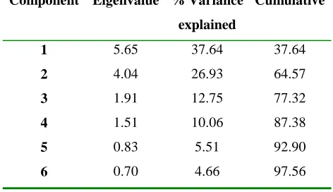
………. Table 3 about here ……….

It can be seen in Table 3 that five eigenvalues take values larger than 0.8, and account for almost 93% of the variance in the data set. This suggests that a map in five dimensions is appropriate. It was decided, nevertheless, to produce the map in six dimensions and treat the last one as residual variation. The importance of the first three principal components is also apparent from the table, which suggests that three characteristics of the data will play a fundamental role in the interpretation of the results.

A set of points in a six-dimensional space is impossible to comprehend. It is necessary to work on projections on pairs of dimensions, but it is possible for two points to be far apart in the space while projecting near to each other in the two dimensions under scrutiny. Arabie et al (1987) recommend that MDS analyses should always be accompanied by cluster analysis, so as to better visualise the results. Chatfield and Collins (1980) are also of the opinion that much is to be gained from visual examination of cluster results.

Following Chang’s (1983) advice that clustering should be conducted using the original data set, fourteen different cluster analyses were performed using Johnson´s (1967) most distant neighbour hierarchical approach, which maximises cluster compactness. Cluster analysis was also performed using other clustering rules, but the results were similar, so they will not be discussed here. The clusters were calculated from the original standardised data, zrlik. As in PCA, a further cluster analysis exercise was conducted with data obtained after averaging ratios over years for individual countries.

A non-hierarchical three-way clustering model due to McLachlan and Basford (1988) was also estimated using the program MIXCLUS3, and the results were found to be identical to those obtained with the traditional clustering method. It was interesting to discover that the non-hierarchical method did not produce overlapping clusters.

The projection of the common map on dimensions 1 and 2 can be seen in Figure 1. The results of cluster analysis using average ratios have been superimposed on this map. Figure 2 shows the projection of the common map on dimensions 1 and 3. The same clusters have been outlined in this figure.

….

Figure 1 about here ….

….

Figure 2 about here ….

A clear division can be observed between the left hand side and the right hand side of Figure 1. The left of this figure contains a cluster formed by Portugal, Italy, Spain, Belgium, and France, to which Finland is attached at a higher level of clustering. The countries to be found on the right hand side of the figure are Sweden, Denmark, Austria, and a later stage in the clustering algorithm, Germany. Holland is also present on this side of the figure, but is best classified as a cluster on its own. Within these clusters there are interesting subclusters; for example, Italy and Spain form an early cluster, as do Belgium and France, and Sweden and Denmark. Another clear partition of the space appears in Figure 2, with one of the main clusters being located at the top left quadrant, and the other one being located at the bottom right quadrant.

ISPBF, includes Italy, Spain, Portugal, Belgium and France; the second group, SDAG, was formed by Sweden, Denmark, Austria, and Germany; the third group, NL, was formed by an individual country, Netherlands; whilst the last group, FL, contains Finland. Finland sometimes appeared to be close to the first group, while Netherlands was always a cluster on its own.

One would be tempted to attach cultural or religious meanings to these findings, but we need to remember that the map has been obtained from company accounts. Does this mean that company accounts are not culture free? Are there two Europes when it comes to company performance? Is it possible that what is being observed is simply the fact that geographical frontiers are in the process of disappearing and that countries that are geographically and culturally close to each other have similar company financial structures? A note of warning was given by Cormack (1971) who said that Cluster Analysis should never be a substitute for clear thinking. Here, statistical methods will be used to assess the reasons why countries cluster the way they do.

The clusters were calculated on the basis of financial ratios but, which ratios determine that a country should belong to a particular cluster? To address this question, only the main two groupings were considered, group ISPBF together with Finland, and group SDAG in which Netherlands had been included. Stepwise Discriminant analysis was used, with Wilk’s lambda as a membership inclusion rule. A 100% classification accuracy was obtained, which is not surprising given the neat way in which countries project on the MDS configuration. The variables that entered in the discriminant function were ratio 3 (financial profitability), ratio 8 (Ratio of interest charges to net turnover), ratio 12 (overall debt ratio), and ratio 14 (debt structure). This suggests that profitability and debt structure are the main reasons why countries cluster the way they do.

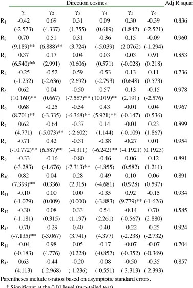
map. If this is the case, it would be possible to draw an oriented line, in the same way as North-South directions are added to geographical maps, so that countries which are further away in the direction of the line are associated with a larger value of the characteristic being represented. For a discussion of this technique see Schiffman et al (1981). The vectors associated with financial ratios have been superimposed on the common map in Figures 3 and 4. Full statistical details are given in Table 4. This table contains standardised cosines for directional vectors,γ_i, t–test statistics with an indication of significance level, and adjusted R2.

The study of Dimension 1 will reveal in what sense cluster SDAG, to the right of this dimension, differs from the other clusters. To do this, one has to examine the vectors that point either to the right or to the left in Figure 3. These are, on the positive side, ratio 2 (net profit/turnover), ratio 3 (return on equity), ratio 5 (Value added/turnover), ratio 6 (staff cost/turnover), ratio 7 (staff cost/value added), ratio 10 (financial results/turnover), and ratio 15 (ratio of provisions for liabilities and charges); and, on the negative side, ratio 8 (interest charges/turnover), and ratio 13 (financial indebtness/balance sheet total). Thus, cluster SDAG is characterised by high levels of net profit, return on equity, value added, and financial results with respect to turnover; this is achieved with high staff cost- reflecting high salaries, high level of provisions- reflecting high pension cost; this is achieved with low interest charges and low levels of debt. Countries in the cluster SDAG, have higher salary levels, which are complemented with schemes for employee’s share in profits, non-provisioned pension funds, and, in general, a legal framework of higher social welfare. The share of personnel cost for German, Danish, and Austrian companies is approximately 25% of turnover, while the European average is 21.7%; European Commission (1998).

tend to borrow short term, and much of the value they add can be attributed to staff cost. The opposite is true of Finland and the Netherlands.

Dimension 3 is associated, on the negative side with the apparent rate of interest on financial debt (ratio 9) and value added over turnover (ratio 5), and on the positive side with share of purchases of goods and services (ratio 4). It can be seen in Figure 2 that cluster SDAG is towards the bottom side of this dimension, while the other clusters are towards the top. We will now comment on these three ratios, as the issues they reveal coincide with a univariate analysis conducted by the European Commission (1998).

The European Commission’s study observes that the purchase of goods and services is the main source of costs for European firms; however, its proportion to total cost varies substantially from country to country. Low cost countries in goods and services are Austria, Germany, and Denmark; high cost countries, reaching up to 70%, are Belgium, Spain, Italy, Netherlands, and Portugal. Three main reasons are given for these differences: the degree of specialisation of the companies involved; different intensity in the use of raw materials; and the extent to which outsourcing takes place. All this is consistent with ratio 4 pointing towards the positive side of Dimension 3. As far as ratio 9 (interest charges to debt owned by financial institutions) is concerned, one has to remember that there are two determinants of financial charges: the level of company indebtness and the interests rates paid by firms. Ratio 9 combines both. It is, in a sense, a measure for cost of capital when funds external to the company are used. If firms are unable to generate enough profitability from their assets to exceed this value, they will face a difficult financial environment. Ratio 5 is one of the best discriminants between the clusters, as it points towards the diagonal from top left to bottom right. This ratio measures vertical integral integration, Morley (1978). This suggests that the cluster SDAG contains companies that are more vertically integrated than companies in cluster ISPBF. According to Morley (1978), companies loose their ability to react to unfavourable economic conditions as they increase their vertical integration.

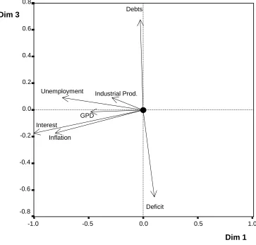
Do the differences in financial structure between the companies that belong to countries in the different clusters reflect different economic environments? This could be either because the economic environment influences the way in which companies work, or because the economy is influenced by the activity of the companies that operate in a particular country. Whichever the reason might be, and the best explanation would be a combination of both, it makes sense to see the relationship between macro-economic variables and the position of the clusters in the configurations. To explore this issue, seven economic variables were treated as properties in a Pro-fit exercise. These variables were the four named in the Maastricht treaty- general government deficit, general government gross debt, inflation, and long term interest rates-; to these were added unemployment, changes in GDP, and changes in the industrial production index. The data was obtained from Eurostat.

Considering that Dimensions 1 and 3 are the main discriminating factors between the clusters, it was not surprising to discover that most of the impact of economic variables was felt in these dimensions. In particular, Dimension 1 was associated with interest rates, inflation, and unemployment on the negative side, indicating that countries that are located towards the left hand side of Dimension 1, the ones in cluster ISPBF, are exposed to higher interest rates, higher inflation, and higher unemployment than countries which are located to the right of this dimension, the countries in cluster SDAG. This is consistent with the findings of Pro-fit analysis using financial ratios, where interest charges were associated with this dimension on the negative side. It is clear that countries that are situated towards the left of this dimension face higher interest rates and this impacts on the profits and losses of the firms. It is also apparent that cluster ISPBF is elongated along Dimension 1, indicating large differences in inflation, interest rates and unemployment between Portugal, at one extreme, and France at the other extreme. Cluster SDAG, on the other hand, is quite compact along dimension 1, indicating that the differences in these economic variables between the countries that are included in the cluster are not very pronounced.

economic variable that has a substantive impact on Dimension 2. Dimensions 4 and 5 appear to be unrelated to economic variables. Figure 5 shows the representation of economic variables on the projection of the common map in Dimension 1 and Dimension 3.

4. CHANGE OVER TIME

In the previous section a static structural analysis has been conducted. This has been based on an exploration of the common map generated by INDSCAL, which represents what has remained constant during the fourteen years under examination. In the INDSCAL model, change is associated with distortions to the common map. Such distortions are obtained by stretching or shrinking the dimensions. The extent to which the distortion is to take place is measured by the weightwdk. It has to be noticed, however, that modifying the map along all the dimensions by the same amount only changes its size. From this it follows that the weights are not important by themselves, what is important is the way in which the relationship between the weights changes over time.

Once the common map has been appropriately modified, a comparison is possible between the original dissimilarity data for a particular year, and what is called the “individual map”. This comparison takes place, as it is often the case in regression, by means of a R2 value. In this particular case, R2 values range from 0.80 to over 0.99, indicating that the time variation in the data is extremely well captured by the model.

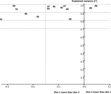
Young Diagrams were calculated for all pairs of dimensions, but only the one which refers to Dimension 1 versus Dimension 3 is shown here in Figure 6. This diagram is chosen for two reasons: first, it has already been established that dimensions 1 and 3 are the ones that best discriminate between clusters; and, second, these dimensions are associated with macro-economic variables, and a business performance cycle can be observed in it. This will now discussed.

Years 1991, 1992, 1993, 1998, and 1999 map on the left hand side of Figure 6. These are years of low economic activity. On the right hand side of this figure we can find years 1988, 1989, 1990, and 1996, which are years of high economic activity. Movements along the horizontal axis are, therefore, related to the business cycle. But, it has to be remembered that the position of the points along the horizontal axis in Figure 6 is determined by the weights associated with the dimensions in the common map. Therefore, the movement of these points reflects the different salience of Dimension 1 versus Dimension 3 for each particular year. This means, that some years the common map has to be stretched along dimension 1 and shrinked along dimension 3, to describe the financial ratios of the firms in the different countries, while in other years this description is obtained by shrinking dimension 1 and stretching dimension 3. In other words, sometimes the ratios associated with dimension 1, such as profitability, become more salient than the ratios associated with dimension 3, such as share of purchases of goods and services. But, if the common map is distorted in this way, the clusters in it are separated or come closer to each other. This means, that the differences that appear over the whole fourteen year period, are accentuated or lessened depending on whether the year under scrutiny is a year of prosperity or depression for the firms. This reaction to the business cycle is clearly reflected in the evolution of the relationships between the weights in the INDSCAL model.

5. CONCLUSIONS

A three-way scaling model, INDSCAL, has proven to be of value to visualise the main features of the data set. This has been done by producing a statistical map (the common map) which shows what remains stable over the fourteen year time period, and a set of weights that explain changes that have taken place over time. The analysis has been supplemented by means of other multivariate methods, such as Linear Discriminant Analysis, Cluster analysis, and Property Fitting- a regression based technique.

The analysis has shown that in European manufacturing industries there exist four clusters which are associated with different financial structures. The cluster formed by Sweden, Denmark, Austria and Germany is characterised by high levels of net profit, value added, and financial results with respect to turnover, achieved through efficiency in purchasing and vertical integration, with high staff costs and high levels of provisions. The converse is true of another large cluster formed by Italy, Spain, Portugal, Belgium and France. Manufacturing companies in Finland and the Netherlands appear to behave in a way which is peculiar to themselves, and these countries form independent clusters.

The clusters have been shown to be robust to the grouping technique employed, and stable over time. The differences between the clusters accentuate at the extremes of the business cycle.

6. REFERENCES

Arabie P., Carroll J.D, and DeSarbo W.S. (1978) Three-way scaling and clustering. Sage University Paper Series on Quantitative Applications in the Social Sciences number 07-065. Beverley Hills: Sage Pubns.

Bailey, K.E., Bylinsky, J.H. and Shields, M.D. (1983). Effects of audit report wording changes on the perceived message. Journal of Accounting Research, 21, 355-370.

Belkaoui, A. (1980). The interprofessional linguistic communication of accounting concepts: an experiment in sociolinguistics. Journal of Accounting Research, 18, 362-374.

Belkaoui, A. and Cousineau, A. (1977). Accounting information, non-accounting information and common stock perception, Journal of Business Finance, 50, 334-343.

Braun, G.P. and Traichal, P.A. (1999). Competitiveness and the convergence of international business practice: North American evidence after NAFTA. Global Finance Journal, 10, 107-122.

Brown, P.R. (1981). A descriptive analysis of select input bases of the Financial Accounting Standards Board. Journal of Accounting Research, 19, 232-246.

Carroll J.D. and Arabie P. (1980). Multidimensional Scaling. In M.R. Rosenzweig & I.W. Porter (editors) Annual Review of Psychology (Vol. 31, pp.607-649). Palo Alto, CA. Carroll J.D. and Chang J.J. (1970). ‘Analysis of individual differences in multidimensional

scaling via an N-way generalization of “Erkart-Young” decomposition’. Psychometrika, 35, 283-319.

Chang, W.C. (1983). On using principal components before separating a mixture of two multivariate normal distributions. Applied Statistics, 32, 267-275.

Chang J.J and Carroll J.D. (1969). How to use INDSCAL, a computer program for canonical decomposition of N-way tables in individual differences in multidimensional scaling. Unpublished manuscript, Murray Hill, NJ; AT & T Bell Laboratories.

Chatfield, C. and Collins, A.J. (1980). Introduction to Multivariate Analysis. Chapman and Hall, London.

Coxon, P.M. (1982). The User's Guide to Multidimensional Scaling. Heinemann, London. Cormack, R.M. (1971). A review of classification. Journal of the Royal Statistical Society,

Series A, 134, 321-367.

European Commission (1997). ‘Financial situation of European enterprises’, European Economy, Supplement A, Economic Trends, No 7, July 1997.

European Commission (1998). ‘Financial situation of European enterprises’, European Economy, Supplement A, Economic Trends, No 11/12. Nov/Dec. 1998.

European Commission (2000). Guide for BACH data users: transition tables between national layout of national accounts and the BACH statements. European Committee of Central Balance Sheet Offices. Brussels.

European Committee of Central Balance Sheet Offices Own Funds Working Group, ECCBSO (1995) Equity of European Industrial Corporations. ECCBSO. European Commission. Frank, W.G. (1979). An empirical analysis of international accounting principles, Journal of

Accounting Research, 17, 593-605.

Gallizo, J.L.; Gargallo, P.; and Salvador, M (2000). The dynamic classification of financial ratios: evidence from Europe of a simplified factor structure. Pp. 193-219 in Cheng F. Lee editor, Advances in Financial Planning and Forecasting, Vol 9. JAI Elsevier. Amsterdam.

Geweke J. (1977). “The Dynamic Factor Analysis of Economic Time-Series Models” in: D.J. Aigner and A.S. Goldberger (eds) Latent Variables in Socioeconomic Models North Holland: Amsterdam.

Goodall, C. (1991). ‘Procrustes methods in statistical analysis of shape’. Journal of the Royal Statistical Society (B), 53, No 2, 285-339.

Green, P.E. and Maheshwari, A. (1969). Common stock perception and preference: an application of Multidimensional Scaling. Journal of Business, 42, 439-457.

Harshman, R.A. (1970). ‘Foundations of the PARAFAC procedure: Models and conditions for an “explanatory” multi-modal factor analysis’. UCLA Working Papers in Phonetics, 16, 1-84.

Jolliffe, I.T. (1972). ‘Discarding variables in Principal Components Analysis’. Applied Statistics, 21, 160-173.

Johnson, S.C. (1967) Hierarchical clustering schemes. Psychometrika, 32, 241-254.

Kiers, H.A.L. (1998). ‘An overview of three-way analysis and some recent developments’. In: A. Rizzi, Vichi, and H.-H. Bock (Eds.), Advances in Data Science and Classification (pp 592-602). Springer. Berlin.

Krzanowski, W.J. (1988). Principles of multivariate analysis. Clarendon Press. Oxford. UK. Libby, R. (1979). Banker's and auditor's perceptions of the message communicated by the audit

report. Journal of Accounting Research, 17, 99-122.

Mar Molinero, C. and Ezzamel, M. (1991). Multidimensional scaling applied to company failure. Omega, 19, 259-274.

Mar Molinero, C., Apellániz, P. and Serrano-Cinca, C (1996). Multivariate Analysis of Spanish Bond Ratings, Omega, 24, (4), 451-462

Markus, G. B. (1979). Analyzing Panel Data. Beverly Hills CA.: Sage.

McLahlan, G.J. and Basford, K.E. (1988). Mixture models: inference and applications to clustering. Marcel Dekker. New York.

McLeay, S. (1986). "The ratio of means, the means of ratios and other benchmarks: an examination of characteristics financial ratios in the French corporate sector", Finance, The Journal of the French Finance Association 7/1, 75-93.

McLeay, S and Fieldsend, S (1987). Sector and size effects in ratio analysis- an indirect test of ratio proportionality. Accounting and Business Research, Spring, 133-140.

Moriarity, S. and Barron, F.H. (1976). Modelling the materiality judgements of audit partners, Journal of Accounting Research, 14, 320-341.

Morley, F.M. (1978). The value added statement. The Institute of Chartered Accountants of Scotland. Gee and Co (Publishers) Ltd. London. UK.

Provan, F. (1993). ‘Review of SPSS version 5 for Windows’. Applied Statistics 42, 686-689. Pruzansky, S. (1975). How to use SINDSCAL, a computer program for individual differences

in multidimensional scaling. Unpublished manuscript, Murray Hill, NJ; AT & T Bell Laboratories.

Rockness, H.O. and Nikolai, L.A. (1977). An assessment of APB voting patterns, Journal of Accounting Research, 15, 154-167 .

Serrano-Cinca, C. and Mar Molinero, C. (2001). Bank failure: a multidimensional scaling approach, European Journal of Finance, 7, (2), 165-183

Schiffman, J.F., Reynolds, M.L. and Young, F.W. (1981). Introduction to Multidimensional Scaling: Theory, Methods and Applications. Academic Press, London.

Countries Data Source

Austria Oestereichische Nationalbank

Belgium Banque Nationale de Belgique / Nationale Bank van België

Denmark Statistics Denmark

Finland Tilastokeskus / Statistics Finland

France Banque de France

Germany Deutsche Bundesbank

Italy Centrale dei Bilanci S.r.l.

Netherlands Centraal Bureau voor de Statistiek

Portugal Banco de Portugal

Spain Banco de España

Sweden Statistiska Centralbyrån / Statistics Sweden

Japan Ministry of Finance

United States Department of Commerce

Definitions of ratios used BACH items

R1. Gross profit ratio

Ratio of gross operating profit or loss to net turnover U/1 R2. Net Profit Ratio

Ratio of net profit or loss for the year to net turnover 21/1 R3. Return on equity

Ratio of profit or loss for the year to equity capital 21/L- A R4. Relative share of purchases of goods and services

Ratio of consumption of goods and services to net turnover 5/1 R5. Value added ratio

Ratio of BACH value added to net turnover T/1 R6. Relative share of staff costs

Ratio of staff costs to net turnover 6/1

R7. Staff costs relative to value added

Ratio of staff costs to BACH value added 6/T

R8. Relative share of financial charges

Ratio of interest charges to net turnover 13/1 R9. Apparent rate of interest on financial debt

Ratio of interest charges to debt owed to credit institutions 13/F2+I R10. Ratio of financial result

Financial result on net turnover W/1

R11. Own funds ratio

Ratio of own funds less unpaid share capital to balance sheet total L- A/FL R12. Overall Debt ratio

Ratio of debt with a remaining period to maturity of more than one year

+ debt with a remaining period to maturity of less than one year to total liabilities F+I/FL R13. Ratio of financial indebtedness

Ratio of financial indebtedness balance sheet total F2+I2/FL R14. Debt Structure

Ratio of debt with a remaining period of maturity of more than one year to debt With a remaining period of maturity of more than one year + debt with a remaining

Period of maturity of less than one year I/I+F R15. Ratio of provisions for liabilities and charges

Provisions for liabilities and charges to balance sheet total J/FL

Component Eigenvalue % Variance

explained

Cumulative

1

2

3

4

5

6

5.65 4.04 1.91 1.51 0.83 0.70

37.64 26.93 12.75 10.06 5.51 4.66

37.64 64.57 77.32 87.38 92.90 97.56

Direction cosines

γ1 γ 2 γ 3 γ 4 γ 5 γ 6

Adj R square R1 -0.42 0.69 0.31 0.09 0.30 -0.39 0.836

(-2.573) (4.337) (1.755) (0.619) (1.842) (-2.521) R2 0.70 0.51 0.31 -0.36 0.15 -0.09 0.960

(9.189)** (6.888)** (3.724) (-5.039) (2.0762) (-1.294)

R3 0.37 0.17 0.04 0.03 0.03 0.91 0.853

(6.540)** (2.991) (0.606) (0.571) (-0.028) (0.218)

R4 -0.25 -0.52 0.59 -0.53 0.13 0.11 0.736

(-1.252) (-2.636) (2.692) (-2.793) (0.648) (0.573)

R5 0.62 0.04 -0.50 0.57 0.13 -0.15 0.978

(10.160)** (0.667) (-7.567)** (10.019)** (2.191) (-2.576)

R6 0.68 -0.25 -0.54 0.43 -0.01 0.04 0.967

(8.701)** (-3.335) (-6.368)** (5.921)** (-0.147) (0.536)

R7 0.62 -0.64 -0.37 0.14 -0.01 0.23 0.899

(4.771) (-5.073)** (-2.602) (1.144) (-0.109) (1.867) R8 -0.71 0.42 -0.31 -0.38 -0.27 0.01 0.954

(-10.772)** (6.587)** (-4.311) (-6.242)** (-4.1921) (0.1923)

R9 -0.33 -0.16 -0.80 -0.46 0.06 0.12 0.891

(-3.283) (-1.676) (-7.313)** (-4.855) (0.582) (1.211) R10 0.82 0.04 0.28 -0.49 0.10 0.06 0.891

(7.399)** (0.336) (2.315) (-4.681) (0.928) (0.597)

R11 -0.10 0.00 0.00 -0.35 0.92 -0.15 0.934

(-1.079) (0.009) (0.000) (-3.883) (9.779)** (-1.626) R12 -0.30 0.08 0.33 0.54 -0.14 0.70 0.585

(-1.181) (0.315) (1.197) (2.261) (-0.567) (2.880) R13 -0.70 -0.29 0.40 0.40 -0.22 -0.25 0.924

(-7.135)** (-3.067) (3.741) (4.377) (-2.238) (-2.732)

R14 -0.04 0.98 0.05 -0.17 -0.07 -0.07 0.704

(-0.183) (4.776) (0.228) (-0.857) (-0.352) (-0.369) R15 0.63 -0.44 -0.20 -0.08 -0.50 -0.35 0.857

(4.113) (-2.968) (-1.236) (-0.551) (-3.313) (-2.393) Parentheses include t-ratios based on asymptotic standard errors.

* Significant at the 0.01 level (two-tailed test). ** Significant at the 0.05 level (two-tailed test).

2 1

0 -1

-2 2

1

0

-1

-2

-3

Dim 1

Dim 2

FRA

°

BEL

°

NLD

°

SPA

°

DNK

°

GER

°

POR

°

SWE

°

AUS

°

ITA

°

Figure 1.

WMDS. Common space. Projection on Dimension 1 and Dimension 2

FIN

2 1

0 -1

-2 2

1

0

-1

-2

-3

Dim 1

Dim 3

FRA

°

BEL

°

NLD

°

SPA

°

DNK

°

GER

°

POR

°

_°

AUS

°

ITA

°

Figure 2.

WMDS. Common space. Projection on Dimension 1 and Dimension 3

°

FIN

Dim 1

0.8 0.4

0.0 -0.4

-0.8

Dim 2

1.0

0.8

0.6

0.4

0.2

0.0

-0.2

-0.4

-0.6

r15

r14

r13

r12

r11

r10

r9

r8

r7

r6

r5

r4

r3

r2

r1

Dim 1

0.8 0.4

0.0 -0.4

-0.8

Dim 3

0.8

0.6

0.4

0.2

0.0

-0.2

-0.4

-0.6

-0.8

r15

r14

r13

r12

r11

r10

r9

r8 _r

7

r6

r5

r4

r3

r2

r1

Dim 1

1.0 0.5

0.0 -0.5

-1.0

Dim 3

0.8

0.6

0.4

0.2

0.0

-0.2

-0.4

-0.6

-0.8

Interest

Figure 5. ProFit Analysis. Mean vectors for each macro-economic variable. Dimension 1 and 3

Deficit GPD

Industrial Prod.

Inflation Unemployment

Dim 3 more than dim 1

0.0 -0.2

Explained variance (r2₎

1.0

0.9

0.8

0.7

0.6

0.5

0.4

0.3

0.2

0.1

86

Figure 6. Young Diagram, Dimension 1 versus Dimension 3

Dim 1 more than dim 3

87 88

89

90 91

92 93

9497 95 ₉₆

98 99