Nondestructive Coupler Characterization Technique
C. Alegria and M. N. Zervas, Member, IEEE
Abstract—A novel nondestructive technique for characterising couplers by means of a local perturbation is described. The method is studied theoretically and verified experimentally by character-ising different types of fused fiber-couplers. Using this technique, both the information of the power distribution and coupling profile along the coupler waist are obtained.
Index Terms—Add–drop multiplexing, coupled mode analysis, coupler fabrication, couplers, optical fiber couplers.
I. INTRODUCTION
F
IBER- and integrated-optic couplers are extremely impor-tant components in a number of photonics applications. They are generally four-port devices and their operation relies on the distributed coupling between two individual waveguides in close proximity, which in turn results in a gradual power transfer between modes supported by the two waveguides. Al-ternatively, the power transfer and cross-coupling at the coupler output ports can be viewed as a result of the beating between the eigenmodes of the composite two-waveguide structure along the length of the composite coupler waist [1]. Fiber- and integrated-optic couplers are used to split the optical power of an optical channel (of certain wavelength) at the output ports (power splitters) [2]. They can also be used to combine or split the power of different channels, corresponding to different wavelengths (wavelength-division-multiplexing (WDM) split-ters/combiners) [3]. Lately, fiber- and integrated-optic couplers have been combined with reflective Bragg gratings, written in their waist, to provide selective adding and dropping of different channels in WDM systems [4], [5].The performance of couplers and coupler-based devices de-pends on the coupling-constant and/or power distribution along the coupling region. The response of coupler-based optical add–drop multiplexers (OADMs) involving Bragg gratings, for example, is critically dependent on the exact positioning of the grating with respect to the points inside the coupler waist where the power on each individual core is equally split [4], or equivalently, the phase difference between the two waist eigenmodes is multiple of . Development of nondestructive coupler characterization techniques, in order to determine the power evolution and coupling constant distribution along the coupler length, is, therefore, of paramount importance in developing couplers for high-performance applications.
Various methods for determining different parameters of uni-form directional couplers have been reported in the literature [6], [7]. Bourbin et al. [6] reported a method for characterising
Manuscript received June 18, 2001. The work of C. Alegria was supported by the Fundação para a Ciência e Tecnologia.
The authors are with the Optoelectronics Research Centre, University of Southampton, Southampton, SO17 1BJ, U.K. (e-mail: [email protected].).
Publisher Item Identifier S 0733-8724(02)05387-2.
couplers in planar waveguides. The method is based on inducing a small differential loss in one of the coupled waveguides. In order to localize the loss perturbation in one of the waveguides only, the other waveguide is covered with a protective resist film. Gnewuch et al. [7] reported an alternative local-perturbation method for measuring the beat-length of uniform couplers in buried planar-waveguide geometry. The method consists of in-ducing a local perturbation in one of the waveguides by heating it with an incident 980-nm semiconductor laser diode. To facili-tate the 980-nm laser absorption by the otherwise transparent waveguides and achieve local heating, a 1- m-thick layer of absorptive black ink was spin-coated onto the coupler surface. The method did not give any results when the coupler was per-turbed symmetrically (laser diode focused at the center between the two waveguides). It should be stressed that the two reported methods require some degree of postfabrication coupler treat-ment (e.g., application of resist film in one of the waveguides [6] and spin-coated absorptive thin-layer [7]) in order to achieve the required differential perturbation. Although such steps and pro-cesses can be acceptable in planar waveguide geometries, they cannot be applied or should be avoided in fused fiber coupler geometries. This is due to the fact that the very small waist di-ameters involved are quite fragile and prone to postfabrication treatment failures.
In this paper, we describe a new nondestructive method for full coupler characterization. The method does not involve any postfabrication treatment and/or extra coupler preparation. First, by applying an asymmetric perturbation between the two lowest order waist eigenmodes, we can nondestructively measure the complex power evolution along the entire coupling region. Fur-thermore, in the particular case of a 100% coupler, the asym-metric perturbation of the coupler provides a marker for the position along the coupler where the power is equally split be-tween both the waveguides (50%–50% point) independently of the wavelength of the light used to monitor the coupler. Second, by applying a symmetric perturbation between the two lowest order waist eigenmodes, we can nondestructively measure the coupling-constant distribution along the entire coupling region.
II. LOCALPERTURBATIONCOUPLERCHARACTERIZATION TECHNIQUE
A. General Description of the Proposed Method
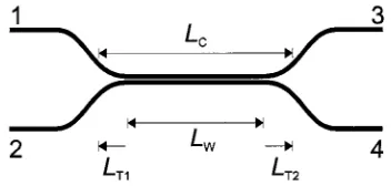
As already mentioned, optical couplers are formed by bringing two or more waveguides (planar, ridge, diffused waveguides, or fibers) in close proximity so that they exchange power through evanescent field interaction. In four-port (2 2) couplers, shown schematically in Fig. 1, two waveguides ex-change powers over a coupling region , which comprises the coupler waist and the two taper regions
Fig. 1. Four-port coupler schematic showing the coupling region(L ), which is comprised of the two taper regions(L ; L ) and the coupler waist (L ).
Fig. 2. (a) Principle of operation of the coupler characterization technique. (b) Schematic of the coupler-waist perturbation using an asymmetric (top) or symmetric (bottom) configuration.
on either side. The taper regions are adiabatic in order to avoid higher order, as well as, radiation mode excitation that con-tribute to losses. The coupling process along the taper lengths is nonuniform, described by a varying coupling constant, and accounts for a substantial part of the total exchanged power. They should, therefore, be taken into account when considering practical coupled devices. The waist region, on the other hand, in most of the cases is supposed to be uniform and is described by a fixed coupling constant. However, in practise, depending on the fabrication process, the waist shows sizeable nonuni-formities that should be properly accounted for, in order to describe accurately the device performance. This is particularly important in more complex devices, such as OADMs, that combine couplers with gratings in their waists [4], [5].
Fig. 2(a) illustrates the principle of operation of the proposed technique. Light of the appropriate wavelength is launched into one of the input ports (#1 or #2). The coupler characteriza-tion method consists of inducing a local perturbacharacteriza-tion along its coupling region (taper waist) and monitoring the change in power (or phase) at one or two of the output ports (#3 and #4). The local perturbation is, in general, induced nondestructively by a temperature gradient across the coupler waist, as shown schematically in Fig. 2. The perturbation (shown by the shaded area) can be asymmetric as in Fig. 2(b)–top or symmetric as in Fig. 2(b)-bottom with respect to the power distribution of even and odd eigenmodes. As it will be shown theoretically and con-firmed experimentally in subsequent sections, the type of the ap-plied perturbation can provide information about different
cou-pler parameters. The temperature gradients were induced by two different techniques, involving different heat sources. The first one was a heated wire and the second one a power-controlled CO laser. The CO laser radiation is highly absorbed by fused silica (typical absorption length of m [11]) and provides the required perturbation gradient without the need for applica-tion of extra absorbing layers (as in [7]).
The method has been first studied theoretically using coupled mode theory, and then demonstrated experimentally, showing excellent agreement. Furthermore, it has been successfully ap-plied to a number of different coupled structures, such as stan-dard fiber fused couplers of different lengths, as well as, com-plex nonuniform coupled fiber structures. The method can pro-vide both the power evolution along the coupler waist and the distribution of the corresponding coupling constant.
B. Theoretical Model
1) Coupler Description: Consider the 2 2 coupler shown schematically in Fig. 1. When light is launched into port#1, the normalized field amplitudes of the even and odd eigenmodes at the coupler input can be approximated by [1]
(1)
where and are the normalized amplitudes of the fields launched initially at the two input ports #1 and #2, respec-tively (see Fig. 1). For single port excitation, and
and, through (1), .
There-fore, light launched into one of the input ports of a 2 2 coupler excites equally the two lowest order (even and odd) eigenmodes along the coupling region. The two eigenmodes propagate adi-abatically along the entire coupling region.
The propagating total electric field at any point along the cou-pler is given by
(2)
During adiabatic propagation, the even and odd eigenmodes
re-tain their amplitude ( and ) and
change only their relative phase. This results in spatial beating along the coupler waist and power redistribution between the two individual waveguides comprising the optical coupler. The peak field amplitudes for each individual waveguide, along the coupling region, can be approximated by [1, Sec. 6.2]
(3)
where
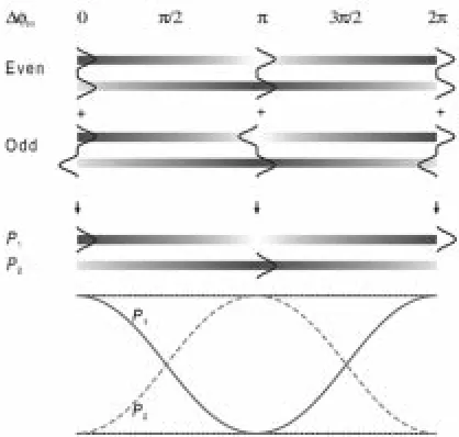
[image:2.612.310.553.622.759.2]Fig. 3. Schematic of even and odd eigenmode beating and total power evolution along a 22 2 full-cycle (1 = 2) coupler.
difference between the even and odd eigenmodes. and are the propagation constants of the even and odd eigenmodes, respectively. The corresponding normalized peak powers carried by the individual waveguides are given
by , namely
(4)
At the points along the coupler, where is zero or multiple of , the total power is concentrated predominantly around wave-guide#1 ( and ). At the points along the coupler, where is multiple of , on the other hand, the total power is concentrated predominantly around waveguide#2 (
and ). Finally, at the points where is multiple of , the total power is equally split between the two waveg-uides . The even/odd eigenmode beating and total power evolution along a full-cycle coupler is shown schematically in Fig. 3. We should add that in case the coupler waist is nonuniform, the irregularities are considered adiabatic so that no power exchange takes place between the two local eigenmodes and/or the radiation modes.
2) Effect of External Perturbation: However, in the presence of a local nonadiabatic (symmetric/asymmetric) externally in-duced refractive index perturbation, at a given distance , the otherwise uncoupled even and odd eigenmodes scatter light into each other and perturb their amplitudes and . The interac-tion between the two propagating eigenmodes can be described by the following coupled-mode equations:
(5)
where . The overall coupling process is character-ized by four parameters, namely and . The pa-rameters and are self-coupling coefficients, describing
Fig. 4. Schematic of even and odd eigenmode self-coupling(k ; k ) and cross-coupling(k ; k ) induced by the external perturbation. The shaded area marks the external perturbation1n.
the scattering of each mode into itself, and result in a modifica-tion of the mode propagamodifica-tion constant locally. The parameters and , on the other hand, are cross-coupling coefficients, describing the scattering of each mode into the other, and give the interaction and power exchange between the even and odd modes. The scattering process and coupling mechanism induced by the external refractive index perturbation (marked by the shaded area), is shown schematically in Fig. 4.
The coupling coefficients can be expressed as
(6)
where is the dielectric permittivity
perturbation. When the refractive index perturbation is uniform across the waist cross section or symmetric with respect to the waist center, the cross-coupling coefficients are zero
. When the refractive index perturbation is antisym-metric with respect to the waist center, the self-coupling coef-ficients are zero . In the general case of an asymmetric perturbation, all coupling coefficients are nonzero. Solving the coupled-mode equations along the local perturba-tion length , we obtain the following expressions for the am-plitudes of the perturbed even and odd mode fields:
[image:3.612.331.528.65.229.2]where
The propagation along an unperturbed coupler region, extended between and , can be described by
(8)
where
(9)
From (7), on the other hand, the propagation along the perturbed region can be put in propagation matrix form as
(10)
where
(11)
where is the average of the
two perturbed propagation constants. The even- and odd-mode
fields at the coupler output and ,
respectively, with the perturbation applied at , are ob-tained in terms of the input fields and
by multiplying the three pertinent propagation matrices and can be expressed as
(12)
The transfer matrix of the perturbation can be further sim-plified by disentangling the coupling event from the propaga-tion process over the perturbapropaga-tion length [12]. The pertur-bation transfer matrix is then expressed as the product of a lo-calized and instantaneous coupling matrix and a simple propa-gation matrix as follows:
(13)
where
and
The error involved in the approximation (13) is and is negligible when the perturbation length is very small.
Substituting (13) into (12) the perturbed fields and of the even and odd modes, respectively, at the cou-pler output can be calculated with the perturbation at . Using the relation (3) the fields of the outputs of the corresponding
in-dividual waveguides and can be calculated.
After simple mathematic manipulations, the power at the out-puts of the corresponding individual waveguides
and are expressed as
(14a)
(14b)
where is the total perturbed phase difference between even and odd modes, expressed as the sum of the total phase difference between the even and odd modes of the
un-perturbed coupler and perturbation term
. The term is the
accumulated phase difference up to the perturbation point and it is therefore a function of . For a uniform coupler, is the only -dependent term. Monitoring the power variation as the perturbation is scanned along the coupler length, we can extract extremely useful information about the coupler waist character-istics and the power evolution along the coupling region. Two different types of perturbation can be considered.
1) Symmetric types, where the perturbation is applied sym-metrically with respect to power distribution of the even and odd eigenmodes. Fig. 2(b)-bottom shows a specific arrangement of symmetric perturbation. From (6), it can be easily deduced that in this case only the self-coupling coefficients and are nonzero while the cross-cou-pling coefficients and are zero.
2) Asymmetric types, where the perturbation is applied asymmetrically with respect to power distribution of the even and odd eigenmodes. Fig. 2(b)-top shows a specific arrangement of asymmetric perturbation. In this case, both the self-coupling and cross-coupling coefficients are nonzero.
a) Symmetric Perturbation
: Under symmetric-perturbation conditions, (14) become
(15)
For an ideal multiple-cycle coupler of length , the unperturbed total phase difference is given by In practice, how-ever, couplers are slightly detuned from the ideal length
( and ). The unperturbed
total phase difference , in this case, is given by
couplers ( even), in the limit of small perturbation , (15) become
(16)
For multiple half-cycle couplers ( odd), the expressions for and are interchanged. From (16), we can see that, in the case of symmetric perturbation, the power leakage at the null port has two contributions. In addition to the initial residual power, due to manufacturing tolerances and errors re-sulting in a small detuning , there exists another term that depends on the difference between the perturbation-in-duced self-coupling coefficients. Although the first contribu-tion is fixed and perturbacontribu-tion independent, the second one, as it will be discussed extensively in Section III-A, depends on the overlap between the perturbation profile induced by the heating element (heating wire, CO laser radiation, etc.) and the even and odd modes of the coupler waist. This overlap is shown to depend on the coupler-waist radius and the perturbation pene-tration depth. Under symmetric perturbation, the power varia-tion on either output port can be used to map the coupling-re-gion outer diameter variation. It can, therefore, provide useful information about the taper-region shape and waist uniformity. In the case of nonuniform couplers (see Section III-B4), it can also provide the exact profile of the entire coupling region. In case of a perfect coupler , the required information
is given by the quadratic term .
b) Asymmetric Perturbation
: In the general case, all coupling coefficients are nonzero. For a slightly detuned coupler with even, and an asymmetric perturbation applied at a position along the cou-pling region, (14) take the form
(17)
where is the total detuning due to the
length mismatch and the perturbation. is the perturbed power leaking at the null port (output port#2) and, for small total
de-tuning and a small perturbation ,
can be approximated by
(18)
The first term of (18) is the residual power at output port#2 due to the small total phase detuning and the nonzero difference between the symmetric perturbation coefficients
[see Fig. 7]. This term is similar to the one appearing under the symmetric perturbation of the coupler [(16)]. The second term depends on the relative position of the applied perturba-tion [through ] and the square of perturbation strength [through ]. From (18) it is observed that for a small phase detuning the power evolution along the coupler is fol-lowed. It can be easily shown that the leaking power acquires maximum values at positions along the coupling region, for which
(19)
The total number of successive maxima is determined by the
relation where . Equation
(19) is also valid for multiple half-cycle couplers where is odd number. In this case, however, the expressions for output powers and in (17) are interchanged. For the related ideal coupler (where ), the corresponding maxima positions fulfil the relation . It can be easily shown that at these positions the total power is split equally between and (50%–50% points). The leaking power acquires min-imum values at the points where the perturbation term in (18) vanishes, i.e., when
(20)
Again for the ideal coupler , at these points the power is concentrated at only one of the waveguides (0%–100% points).
3) Asymmetric Perturbations of Nonideal Couplers: From (19) it is deduced that the presence of a finite phase detuning introduces an error in the determination of the 50%–50% points. The detuning of the coupler may be caused by the following.
a) Maintaining the Coupler Strength and Varying the Cou-pler Length: For uniform couCou-plers the error in the determina-tion of the 50%–50% points of the coupler (at the resonance) due to a phase detuning originated by varying the coupler length to while maintaining the strength of the coupler is given by
(21)
where are the actual 50%–50% points of the ideal coupler and are the maxima of the nonideal asymmetric perturba-tion. This error can be minimized by launching light with a wavelength close to the resonance wavelength of the coupler and using a very small perturbation. For a full-cycle coupler with 20-dB extinction ratio and a length of 30 mm, the error in the 50%–50% point positions is mm.
b) Varying the Coupler Strength and Maintaining the Cou-pler Length: This situation arises when characterising the cou-pler at a different wavelength (test wavelength, ) than the res-onance wavelength, . For full-cycle couplers, at the test
wavelength, , we have . We assume that is very close to and therefore is considered constant. The coupler phase displacement from the resonance is
given by where is the length of the
coupler. For a test wavelength of we have and if we have . If the coupler is characterized at the resonance wavelength then and . It can be easily shown that, for a uniform full-cycle coupler the error in the 50%–50% points due to a phase detuning is given by
(22)
where correspond to the first and second 50%–50% point, respectively, and corresponds to the position of the 50%–50% point of the ideal coupler and are the maxima of the nonideal asymmetric perturbation. It is interesting to note that the (0%–100%) point of the coupler corresponds to the min-imum of the perturbation independently of the phase detuning . When calculating the error between the local minimum of the asymmetric perturbation given by (20) and the position of the (0–100%) point of the full-cycle coupler we find
(23)
For a uniform half-cycle coupler the error in the 50%–50% points due to a phase detuning is given by
(24)
Therefore, for a half-cycle coupler the maximum of the leaking power due to an asymmetric perturbation is a marker of the 50%–50% point of the coupler independently of the phase de-tuning of the coupler i.e., independent of the test wavelength.
4) Output Relative Phase Measurements: The asymmetric perturbation of the coupler will also affect the electric field phase at the output ports. The phase of the output light of the perturbed coupler will vary with the perturbation posi-tion along the coupler waist. The output phase is given by
, where is the field
amplitude at the output port#1 or port#2. From (10), and for a perfect full-cycle coupler the phase change at the output port in relation to the unperturbed coupler is given by
(25)
For small perturbations the phase difference is approximated by
(26)
From (4) it is then deduced that, with the perturbation applied at position , the relative phase change of the field amplitude at output port#1 is proportional to the individual-waveguide power . Therefore, the change in the relative phase of the field at the coupler output maps directly the power evolution along the corresponding individual waveguide. This information can be
used to calculate the coupling constant distribution along the coupling region. For a perfect full-cycle coupler
no light arrives at port#2 and therefore the phase displacement cannot be measured at that port.
In the case of nonideal full-cycle couplers with a slight phase detuning phase change at the output port in due to the asymmetric perturbation of the coupler is given by
(27)
For full-cycle couplers with a small phase detuning, the phase change at output port#1 continues to map the power evolution along the coupler. However, the phase change at output port#2 does not provide a direct measurement of the coupler power evolution, as shown in (27).
III. NUMERICALSIMULATIONS
A. Overlap Integrals Between the Coupler Eigenmodes and the Perturbation Profile
Characterization of couplers using a symmetric and asym-metric perturbation allows the location of the 50%–50% power points of the coupler and measurement of the beat length as well radius nonuniformities in the taper profile. The perturbation can be induced by a number of localized heat sources, such as ex-ternal heating elements or illumination by light sources (white light, CO laser, He–Ne laser, laser diodes, etc.). The various sources will induce different perturbation profiles and therefore will have a different overall effect.
In order to investigate the effectiveness of the perturbation we consider a simplified phenomenological model in order to calculate the relative magnitude of the coupling coefficients . The highly fused coupler waist is first approximated by a circular cross-section glass structure with negligible core. The coupler modes are approximated by the lowest order modes ( and ) of this multimode cladding-air structure [9], [10]. The coupler is perturbed locally by radiation incident from side (symmetric perturbation) and side (asymmetric perturbation), as shown in Fig. 5. The absorption of the radiation generates instantaneous heating of the structure that follows an exponential decay across the waist. This results in a local change of the refractive index
of the structure by . According to [1],
for fused silica, the coefficient K .
For the CO radiation, typical value for the penetration length is – m [11]. Fig. 6 illustrates the symmetric and asymmetric perturbation of a coupler with a radius of 30 m and a radiation penetration length of m.
The perturbation is quantified by calculating the overlap in-tegrals between the temperature distribution and the mode profiles. The overlap integrals are defined by
Fig. 5. Perturbation of a 30–m coupler by CO radiation. Left: Symmetric perturbation configuration: Right: Asymmetric perturbation configuration. Top: Even mode profile. Middle: Odd mode profile. Bottom: temperature distribution
f(x; y) across the fiber.
Fig. 6. Coupling coefficient variation with the absorption length of the incident radiation for a coupler waist radius of 16m. Dashed lines: Symmetric perturbation. Solid lines: Asymmetric perturbation.
and, therefore, the overlap integrals are pro-portional to the coupling coefficients .
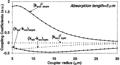
[image:7.612.308.549.64.194.2] [image:7.612.44.288.350.480.2]We first consider the effect of the radiation penetration depth on the coupling coefficient magnitude, for symmetric and asymmetric perturbation. The coupler waist radius is consid-ered to be 16 m, which is typical of the devices we routinely fabricate with a flame brush technique. Fig. 6 shows the relative variation (in arbitrary units) of the coupling constant and the corresponding difference , under symmetric (dashed lines) and asymmetric perturbations (solid lines), for different radiation absorption lengths. It should be reminded that under pure symmetric perturbation (Section II-B2.1), the perturbed output power is proportional to the difference [see (16)], while under pure asymmetric pertur-bation Section II-B2.2, the perturbed power is proportional to [see (18)]. Fig. 6 shows that both asymmetric-perturbation and symmetric-perturbation are maximized for a range of absorption lengths between 10 m and 17 m, i.e., the proposed perturbation method is optimized for radiation
Fig. 7. Coupling coefficient variation with coupler-waist radius. The perturbing radiation absorption length was 5m (typical of CO laser). Dashed lines: symmetric perturbation. Solid lines: asymmetric perturbation.
absorption lengths comparable to the coupler waist radius. Fig. 6 also shows that asymmetric perturbations result in finite , which nevertheless, is appreciably smaller than the accompanying . Under symmetric perturbation, as expected, is negligible for every absorption length. Finally, as the absorption length is increased appreciably the perturbation becomes increasingly uniform across the entire coupler waist cross-section and all the parameters tend to zero, under either perturbation. This suggests that the proposed nondestructive perturbation method would not work in case the perturbing radiation was provided by a He–Ne laser at 633 nm (absorption length in silica m) or any other visible or near-infrared laser (with absorption lengths well above the waist diameter). Use of radiation with large absorption length would have required application of an extra highly absorbing layer (as in [7]), which is not applicable in our case.
Next, in Fig. 7, we consider the variation of the coupling co-efficients and the differences for different cou-pler-waist radii, under CO laser symmetric (dashed lines) and asymmetric (solid lines) side-perturbation. For the calculations, we have considered a typical absorption length of 5 m. As be-fore, the asymmetric-perturbation and symmetric-perturba-tion are maximized for a coupler waist of about 5 m, i.e., comparable to the radiation absorption length. Fig. 7 also shows that for small coupler-waist radii, asymmetric pertur-bations result in appreciably smaller than the accom-panying . However, for larger coupler-waist radii, the differ-ence becomes comparable with and finally equal to and the simple analytic formula (18) is not valid any more. In this case, the power perturbation at the coupler output should be calculated using (14a) and (14b). Again, under symmetric perturbation, is zero for every coupler-waist radius.
Fig. 7 shows that, under symmetric perturbation, the differ-ence changes quasilinearly with the coupler-waist radius. From (16), it is then obvious that output power pertur-bation will follow closely the coupler-waist outer diameter as the CO laser is scanned along the coupling region. The output power variation can then provide a reliable mapping of the en-tire coupling region giving a quite accurate estimation of the coupler uniformity.
Fig. 8. Coupling coefficient variation with the power of the incident CO laser radiation under asymmetric perturbation. The perturbing radiation absorption length was 5m and the coupler waist radius was 16 m.
varying coupling region, in addition to the expression in paren-theses of the second term, the perturbation output power is ap-propriately weighted by the varying coefficient. In addition, if the is larger or comparable to (for large cou-pler-waist radii or under weak CO laser power), the significant
term in (18) should also be taken into account. In Fig. 8 we consider the effect of different incident radiation powers on the magnitude of the coefficients and under asymmetric perturbation. We assume that there is a linear dependence of the refractive index with the power of the incident radiation and therefore, the coupling coefficients
and are proportional to the power of the incident radiation. The absorption length of the incident radiation was 5 m (CO laser radiation) and the coupler waist radius was 16 m. For high powers of the CO laser (region 3 in Fig. 8),
and the asymmetric perturbation of the coupler can be used to locate the 50%–50% points of the coupler. For small values of
the CO laser power where or
(regions 1 and 2 in Fig. 8, respectively) the first term in (18) should be taken into account.
B. Coupler Perturbation Results
In order to verify the approximate results [given by (16) and (18)], an exact model based on the transfer-matrix method was implemented. The entire coupler is divided in uniform sec-tions and the transfer matrices corresponding to each section were calculated using (8) to (10). The transfer matrix of the en-tire coupler is then easily calculated by multiplying the indi-vidual transfer matrices. No simplifications to the perturbation matrix where made. In this model, any coupling profile can be introduced and both the symmetric and asymmetric perturba-tions can be accounted for by modifying the values of the cou-pling coefficients and . A number of different cou-pler configurations were considered with coupling coefficient profiles of varying complexity. They are intended to prove that for all coupling coefficient geometries, an asymmetric pertur-bation scanned along the coupling region always provides the 50%–50% power points. In the following simulations we con-sider an ideal asymmetric perturbation with only the perturba-tion coefficient being nonzero.
[image:8.612.317.537.63.209.2]1) Uniform Coupler: The first simulation refers to an ideal uniform coupler with constant coupling coefficient throughout the coupling region. The total coupler length is mm. The
Fig. 9. Normalized power evolution along each “individual” waveguide (dashed lines), as well as, output power perturbation (solid line) as a function of the perturbation position along the coupling region of an ideal uniform coupler. The coupling coefficient profile is also superimposed for better visualization.
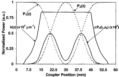
Fig. 10. Normalized power evolution along each “individual” waveguide (dashed lines), as well as, output power perturbation (solid line) as a function of the perturbation position along the coupling region of a uniform coupler with two tapered regions. The coupling coefficient profile is also superimposed for better visualization.
total phase difference between the even and odd eigenmodes was (full-cycle coupler). Fig. 9 shows the nor-malized power evolution and of each “individual” waveguide (dashed lines), as well as, the output power perturba-tion (solid line) as a function of the perturbation posi-tion along the coupling region. The coupling coefficient profile is also superimposed for better visualization.
These results illustrate that the positions in the coupler, where the output power perturbation is maximum, correspond to the points where the power is equally distributed between the two
“individual” waveguides . For an ideal
uniform coupler of length , these points are situated at and . The simulation results show that the 50%–50% points are at 7.5 mm from the centre of the coupler, as expected.
[image:8.612.313.538.268.414.2]Fig. 11. Normalized power evolution along each “individual” waveguide (dashed lines), as well as, output power perturbation (solid line) as a function of the perturbation position along the coupling region of a uniformly-tapered coupler (small taper ratio). The coupling coefficient profile is also superimposed for better visualization.
Fig. 12. Normalized power evolution along each “individual” waveguide (dashed lines), as well as, output power perturbation (solid line) as a function of the perturbation position along the coupling region of a uniformly tapered coupler (extreme taper ratio). The coupling coefficient profile is also superimposed for better visualization.
show that the effect of the taper region on the power distribution along the coupler is to move the 50%–50% points away from the center of the coupler due to some coupling between the modes in the transition region. The results also illustrate that the maxima of the output perturbation power coincide with the 50%–50% points, which are placed 9.5 mm away from the center of the coupler.
3) Uniformly Tapered Coupler: We next consider some ex-amples of nonuniform couplers. First, we study a uniformly ta-pered coupling coefficient profile, with small taper ratio. These profiles can be encountered in real fused couplers and may be due to temperature nonuniformities along the fused waist or other experimental inaccuracies. The results of the simulation are shown in Fig. 11. Fig. 12 shows the simulated perturbation results of a uniformly tapered coupler with extreme taper ratio. In both cases, the total coupler length was mm and the total phase difference between the even and odd eigenmodes
was (full-cycle coupler).
Despite the different individual power distributions, in both cases, the output power perturbation maxima coincide with the points along the coupler where the power is split equally
be-Fig. 13. Normalized power evolution along each “individual” waveguide (dashed lines), as well as, output power perturbation (solid line) as a function of the perturbation position along the coupling region of a nonuniform coupler (MZI). The coupling coefficient profile is also superimposed for better visualization.
tween the two “individual” waveguides .
4) Nonuniform Coupler (Mach–Zenhder Interferom-eter): The final simulation concerns a complex nonuniform coupling structure constituted by two weakly coupled re-gions and an intermediate uncoupled region. The length of each weakly coupled region is mm and the total coupler length mm. The phase difference between the even and odd eigenmodes along each weakly coupled
region is . The total phase
differ-ence between the even and odd eigenmodes, in this case, is (half-cycle coupler). Since the coupler is half-cycle long, the perturbation is measured at the output of waveguide#1. Fig. 13 shows the normalized power evolution and of each “individual” waveguide (dashed lines), as well as, the output-power perturbation (solid line) as a function of the perturbation position along the coupling region. The coupling coefficient profile is also superimposed for better visualization.
At the end of the first weakly coupled region, the power is equally split between the “individual” waveguides #1 and #2 . The powers remain unchanged over the central uncoupled region and cross-couple completely at the end of second weakly coupled region. The output-power perturbation (solid line) maps exactly this power evolution. It is shown that reaches a maximum value when the per-turbation reaches the end of the first weakly coupled region and retains it over the entire uncoupled central region. It is easily realized that this complex coupled structure corresponds to a Mach–Zenhder interferometer (MZI).
C. Perturbations of Nonideal Couplers
As already mentioned in Section II-B3, in the presence of a finite detuning the perturbation power maxima are displaced from the actual 50%–50% power points by an amount given by (21) or (22) depending on the nature of the phase detuning.
[image:9.612.53.278.286.432.2]Fig. 14. Asymmetric perturbation of full-cycle couplers for different detuning values(1 = 0; 60:21) achieved by using different lengths for each coupler. The asymmetric coupling contribution remained constant,k 1z = 0:22. Thick lines: Power distribution along the coupler. Thin lines: Perturbation of the detuned couplers. Dashed line: Perturbation of the ideal coupler. (The perturbation power is multiplied by a factor of ten).
from the optimum point, ( is considered
zero). The thick solid lines show the power evolution along the coupler length. The dashed line shows the asymmetric perturbation of the ideal coupler, while the thin solid lines show the corresponding perturbations of the detuned cou-plers. The shifts in the perturbation maxima from the ideal case [see (21)] are clearly shown. In these simulations, the coupling strength remained constant and the phase displace-ment, , was achieved by varying the coupler length by mm. The length of the ideal
coupler was mm and the coupling strength
of all couplers was . In these simulations the cross-coupling coefficient remained constant,
and .
For a uniform coupler with a coupling strength of where mm is the optimum coupler length and for a phase displacement of , the correction to the perturbation maxima positions, in order to obtain the 50%–50% points of the coupler is given by (21),
mm.
2) Varying the Coupler Strength and Maintaining the Coupler Length: In the following simulations, the coupling length remained constant and the phase displacement, , was achieved by varying the difference between the coupler eigenmodes by . As already mentioned, this phase detuning could be achieved by characterizing the coupler at a wavelength different from its resonance wavelength.
Fig. 15 shows the simulation of the asymmetric perturba-tion of a uniform full-cycle coupler with different phase dis-placements. Fig. 15(a) shows the power evolution (solid lines) and asymmetric perturbation (dashed line) of an ideal coupler tested at the resonance wavelength . The vertical dashed lines show the positions of the asymmetric-per-turbation maxima that coincide with the actual 50%–50% points of the coupler (shown by the arrows). Fig. 15(b) and (c) show the corresponding power evolution (solid lines) and asymmetric perturbation (dashed lines) of the coupler tested at the
wave-lengths and ,
respectively. The vertical dashed lines show the corresponding asymmetric perturbation maxima which now differ from the ac-tual 50–50% points of the ideal coupler (marked by the arrows).
Fig. 15. Asymmetric perturbation of full-cycle couplers for different detuning values(1 = 0; 60:3) achieved by using different coupling strengths for each coupler. The arrow markers correspond to the 50%–50% points of the ideal coupler and the dashed lines to the maxima of the asymmetric perturbation. (a) Power evolution and perturbation of the ideal coupler(1 = 0). (b) Power evolution and perturbation of a coupler detuned by1 = +0:3. (c) Power evolution and perturbation of a coupler detuned by1 = 00:3. (The perturbation power is multiplied by a factor of ten.
In accordance with expression (22) the perturbation maxima in these cases are shifted inside or outside
of the actual 50%–50% points. Both the magnitude and the di-rection of this shift should be accounted correctly in order for the actual 50%–50% points to be retrieved. It should also be stressed that in all cases the (0%–100%) point (given by the asymmetric perturbation minimum) remains fixed as the theory predicts (expression 23). In these simulations the difference be-tween the eigenmodes of the ideal coupler was and the length of all couplers was mm. The difference between the eigenmodes of the detuned couplers
was . The cross-coupling coefficient
re-mained constant, and .
For a uniform coupler with a length mm, where is the optimum coupling strength and for a phase displacement of , the correction to the perturbation maxima positions, in order to obtain the 50%–50% points of the ideal coupler are given by,
and . It can be seen that the
corrections are different for ( mm
and mm) and ( mm
[image:10.612.73.257.62.181.2]Fig. 16. Asymmetric perturbation of half-cycle couplers for different detuning values(1 = 0; 60:2) achieved by using different coupling strengths for each coupler. The arrow markers correspond to the 50%–50% point of the coupler and the dashed lines to the maxima of the asymmetric perturbation. (a) Power evolution and perturbation of the ideal coupler(1 = 0). (b) Power evolution and perturbation of the coupler detuned by1 = +0:2. (c) Power evolution and perturbation of the coupler detuned by1 = 00:2. (The perturbation power is multiplied by a factor of ten).
different phase displacements. Fig. 16(a) shows the power evo-lution (solid lines) and asymmetric perturbation (dashed line) of an ideal coupler tested at the resonance wave-length . The vertical dashed line shows the posi-tion of the asymmetric-perturbaposi-tion maximum that coincides with the actual 50%–50% point of the coupler (shown by the arrow). Fig. 16(b) and (c) show the corresponding power evolu-tion (solid lines) and asymmetric perturbaevolu-tion (dashed lines) of
the coupler tested at the wavelengths and
respectively. The vertical dashed lines show the corresponding asymmetric perturbation maximum that still coincide with the actual 50%–50% points of the ideal cou-pler (marked by the arrows) as predicted by the theory (expres-sion 24). In these simulations the difference between the
eigen-modes of the ideal coupler was and
the length of all couplers was mm. The difference between the eigenmodes of the detuned couplers was
. The cross-coupling coefficient remained constant,
and .
The correction to the maximum of the asymmetric perturba-tion of a half-cycle coupler [given by (24)] is zero and therefore it is a marker to the 50%–50% point of the half-cycle coupler independently of the coupling strength of the coupler or
equiv-Fig. 17. Simulation of the phase displacement at port#1 due to an asymmetric perturbation of a full-cycle coupler. The dashed lines refer to the power distribution along the coupler. The solid line refers to the phase shift relative to the unperturbed case.
alently, independently of the wavelength at which the coupler is characterized as long as .
Finally, it should be stressed that in the case that the coupler waist is twisted, as the perturbing element is scanned along the coupler length results in both symmetric and asymmetric per-turbation with mixed results that do not provide any useful in-formation.
D. Output Phase Perturbation
In Section II-B4 it was shown analytically that for a perfect coupler under pure asymmetric perturbation , the phase of the electric field at the output port with nonnull power [given by (25)] is proportional to the power of the corresponding “individual” waveguide at the point of the perturbation. There-fore, the output phase variation maps directly the power evolu-tion along the corresponding “individual” waveguide.
The phase change due to an asymmetric perturbation was simulated for an ideal uniform full-cycle coupler
by using expression (12). The asymmetric cross-perturbation coefficient was and the self-perturbation coef-ficients were considered zero . The results of the simulation in Fig. 17 show that the phase variation of the electric field at the output of the “individual” waveguide#1 (solid line) follows indeed closely the power evolution along the corresponding “individual” waveguide. For an optimum cycle coupler with light launched in port1, the coupling profile can be obtained by measuring the output phase at the same port. The output phase changes can be accurately mea-sured by using a phase sensitive (interferometric) technique.
IV. EXPERIMENTALRESULTS
[image:11.612.325.534.62.193.2]Fig. 18. Experimental setup for the characterization of couplers using a perturbation induced by a CO laser.
perturbations. Subsequently, the perturbation was induced by scanning across the coupler waist the output of a CO laser at 10.6 m. This technique proved to be much more stable, re-peatable and accurate. In order to accurately measure the per-turbation, the laser output was modulated and the power os-cillations due to the perturbation where detected and amplified using a lock-in amplifier. The experimental setup is illustrated in Fig. 18.
Light is launched in the coupler through port1 at 1.55 m using a DFB-LD and the light arriving at port3 and port4 is detected and amplified using a lock-in amplifier. A mirror is mounted on a translation stage in order to scan the CO laser across the coupler waist. A symmetric perturbation is induced to the coupler by shining the CO laser perpendicularly to the two cores [see Fig. 2(b)]. An asymmetric perturbation of the coupler is accomplished by rotating the coupler by 90 around its axis.
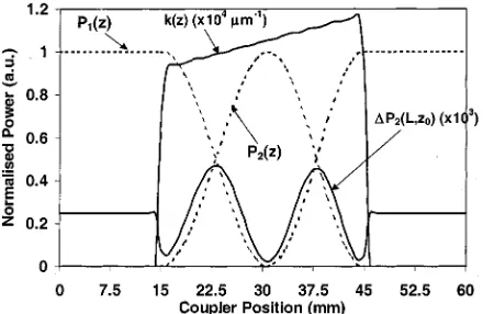
Several experiments were performed in order to prove the theoretical predictions mentioned before. Three different cou-plers where fabricated and characterized using the perturbation method: a half-cycle coupler , a full-cycle coupler and a complex nonuniform coupler. The length for all these couplers was 30 mm, however, they are all approx-imately twice that length due to a long transition region. Both the symmetric perturbation and asymmetric perturbation where used to characterize the couplers.
A. Characterization of a Half-Cycle Coupler
These couplers transfer light from one fiber to the other (light that is launched into port1 exits at port4) has one point where the power is equally distributed in both fibers that should be local-ized in the center of the coupler. Under asymmetric perturba-tion, the perturbed power will peal once at the 50%–50% point. The results of the characterization of a coupler are shown in Fig. 19. The asymmetric perturbation the power distribution along the coupler and the symmetric perturbation follows the coupling profile. The symmetric perturbation was normalized to and used as the coupling profile to fit theoretically the asym-metric perturbation (Fig. 19). Although the symasym-metric
[image:12.612.50.280.67.249.2]perturba-Fig. 19. Characterization of a coupler using the symmetric and asymmetric perturbation. The asymmetric perturbation was fitted using the coupling profile retrieved from the symmetric perturbation data.
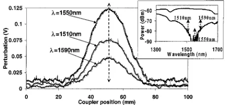
Fig. 20. Characterization of a half-cycle coupler a three different wavelengths ( = 1510 nm, = 1550 nm and = 1590 nm) using an asymmetric perturbation. The small figure is the measured spectral response of the characterized coupler and the markers correspond to the characterized wavelengths.
tion follows the difference between the self-coupling perturba-tion coefficients, , it will match closely the coupling profile, of the measured coupler differing mainly in the ta-pered regions.
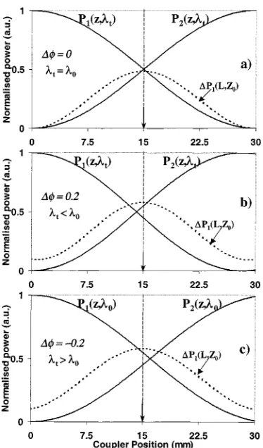
In Sections II-B3 and III-C it was mentioned that the max-imum of the power change, due to an asymmetric perturbation, is a marker for the 50%–50% points of the coupler indepen-dently of the small phase detuning of the coupler (either due to strain in the mounting of the coupler or the characteriza-tion at a wavelength different from the coupler resonance wave-length). This information is very useful since the 50%–50% points of half-cycle couplers can be always obtained with using a normal laser diode to characterize the coupler and without the need of a tunable laser set to the coupler exact resonance wave-length. In Fig. 20 experimental results of the characterization of a half-cycle coupler at different wavelengths are shown. A tunable laser was used to launch light in the coupler port#1 in-stead of the DFB-LD as shown in experimental setup (Fig. 16). Three different test wavelengths where used: nm,
nm (coupler resonance wavelength) and
nm. The power of the CO laser was the same for all the exper-iments (100 mW through a 2-mm pinhole).
[image:12.612.315.539.260.364.2]Fig. 21. Characterization of a2 coupler using the symmetric and asymmetric perturbation. The asymmetric perturbation was fitted using the coupling profile retrieved from the symmetric perturbation data.
differences in the tunable laser output power at the three wave-lengths.
B. Characterization of a Full-Cycle Coupler
As shown in Fig. 9, the asymmetric perturbation of a full-cycle coupler has two maxima that correspond to the 50%–50% power points of the coupler. The fabricated coupler was characterized using both the symmetric perturbation and asymmetric perturbation. As for the case of the half-cycle coupler, the coupling profile obtained from the symmetric perturbation was used to fit theoretically the asymmetric perturbation response. The experimental and theoretical results are in good agreement (Fig. 21). The symmetric perturbation resulted in a very weak and therefore noisy after amplification signal. The experimental asymmetric perturbation has two points where the power of the perturbation is a maximum. However, there is a slight difference in the height of the two peaks accompanied by a variation of symmetric-perturbation signal. This can be due to a small variation of the coupler waist outer diameter or a slight waist twist. A small misalignment between the coupler waist and the scanning CO could also produce similar asymmetries. The asymmetric perturbation was fitted assuming a linear variation of 5% in the asymmetric coupling coefficient from waist end to end. The mean value is
supposed to be m .
In order to prove that asymmetric perturbation of the cou-pler follows the coupling profile for weak perturbations ( very small) and follows the power distribution in the coupler for large (as referred in Section III-A), a coupler was characterized using different CO laser powers (Fig. 22). The laser output powers used were 30, 42, and 96 mW. The actual power that hits the fiber is much lower, given approximately by the ratio of outer waist diameter ( m) over the unfocused laser spot size ( mm). To reduce the spot size of the CO laser and increase the resolution of the method, a 1 mm aperture was used, reducing the power hitting the coupler
to of the output power.
[image:13.612.46.286.63.204.2]From Fig. 22, for a CO laser power of 30 mW the asym-metric perturbation seems to follow the coupling profile of the structure and no maxima (50%–50% points) are observed. This situation corresponds to region-1 in Fig. 8. By increasing the power to 42 mW, an intermediate response is observed where
[image:13.612.315.544.244.371.2]Fig. 22. Characterization of a2 coupler using the asymmetric perturbation for different powers of the CO laser.
Fig. 23. Experimental characterization of a complex nonuniform coupler using a symmetric and asymmetric perturbation.
the two perturbation maxima start arising and the coupling pro-file effect is stronger due to the increase of the coef-ficient as well. At this power the magnitude of the coefcoef-ficients and is comparable (corresponding to region-2 of Fig. 8). For slightly larger powers of the CO laser (96 mW), the coefficient is predominant and the power distribution in the coupler is followed (region-3 of Fig. 8). The correction in the position of the 50%–50% points of the coupler in relation to the maxima of the asymmetric perturbation due to a phase detuning of the coupler and the coefficient can be determined by (22).
In Fig. 22 it is observed that using the asymmetric configura-tion, there is a threshold in the CO laser power in order to track the power distribution of the coupler and identify the 50%–50% positions.
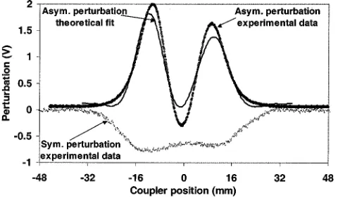
C. Characterization of a Complex Nonuniform Coupler
coupling regions and a region with low coupling strength in the middle. The profile may be distorted due to averaging of the ideal profile by the size of the flame, by noise while character-ising the structure and also by a tilt in the CO laser position along the coupler. The asymmetric perturbation was also char-acterized by rotating the fiber by 90 . The result (Fig. 23) shows an increase of the perturbation until the uncoupled region and then a decrease in the second coupling region. The slight tilt in the perturbation is probably due to a change in along the cou-pler. However, when compared to the theoretical results shown in Fig. 23, the experimental data are in very good agreement.
V. CONCLUSION
A full description of a method of nondestructively character-ising uniform and nonuniform fiber couplers was described. The method consists in perturbing locally a fiber coupler using a CO laser radiation or other radiation with a penetration length close to the coupler diameter. By inducing a symmetric perturbation with respect to the two lowest order waist eigenmodes, useful in-formation about the taper profile and uniformity of the coupler waist can be obtained. By inducing an asymmetric perturbation, on the other hand, the power evolution along the entire coupling region can be followed. Additional information may be obtained by measuring the output electric field phase in the case of the asymmetric and symmetric perturbations. The method can used for the optimization of add–drop multiplexers based on different coupler structures with inscribed gratings. It can also be used in industrial facilities for the identification of errors and optimiza-tion of the fabricaoptimiza-tion procedure of fiber couplers (power splitters or WDM couplers) by the suitable characterization of the devices.
ACKNOWLEDGMENT
The authors thank R. Feced for useful discussions.
REFERENCES
[1] D. Marcuse, Theory of Dielectric Optical Waveguides, 2nd ed. New York: Academic, 1991, ch. 6.
[2] B. S. Kawasaki, M. Kawachi, K. O. Hill, and D. C. Johnson, “Single-mode-fiber coupler with a variable coupling ratio,” J.
Light-wave Technol., vol. LT-1, pp. 176–178, Mar. 1983.
[3] A. Lord, I. J. Wilkinson, A. Ellis, D. Cleland, R. A. Garnham, and W. A. Stallard, “Comparison of WDM coupler technologies for use in er-bium-doped fiber amplifier systems,” Electron. Lett., vol. 26, no. 13, pp. 900–901, June 21, 1990.
[4] F. Bakhti, P. Sansonetti, C. Sinet, L. Gasca, L. Martineau, S. Lacroix, X. Daxhelet, and F. Gonthier, “Optical add/drop multiplexer based on UV-written Bragg grating in a fused 100% coupler,” Electron. Lett., vol. 33, no. 9, pp. 803–804, 1997.
[5] F. Bakhti, X. Daxhelet, P. Sansonetti, and S. Lacroix, “Influence of Bragg grating location in fused 100% coupler for add and drop multiplexer realization,” in OFC—Tech. Dig. Ser., 1998, pp. 333–334.
[6] Y. Bourbin, A. Enard, M. Papuchon, and K. Thyagarajan, “The local absorption thechnique: A straightforward characterization method for many optical devices,” J. Lightwave Technol., vol. LT-5, pp. 684–687, May 1987.
[7] H. Gnewuch, J. E. Roman, M. Hempstead, J. S. Wilkinson, and R. Ul-rich, “Beat-length measurement in directional couplers by thermo-optic modulation,” Opt. Lett., vol. 21, no. 15, pp. 1189–1191, Aug. 1996. [8] M. K. Davis, M. J. F. Digonnet, and R. H. Pantell, “Thermal effects in
doped fibers,” J. Lightwave Technol., vol. 16, pp. 1013–1023, June 1998. [9] A. W. Snyder and J. D. Love, Optical Waveguide Theory. London,
U.K.: Chapman and Hall, 1983.
[10] A. W. Snyder and X. H. Zheng, “Optical fibers of arbitrary cross sec-tion,” J. Opt. Soc. Amer. A, vol. 3, pp. 600–609, 1986.
[11] N. Sahba and T. J. Rocket, “Infrared absorption coefficients of silica glasses,” J. AmER. Ceram. Soc., vol. 75, pp. 209–212, 1992. [12] R. Feced and M. N. Zervas, “Efficient inverse scattering algorithm for
the design of grating-assisted codirectional mode couplers,” J. Opt. Soc.
Amer., vol. 17, no. 9, pp. 1573–1582, Sept. 2000.
C. Alegria was born in Mozambique on May 1,
1973. He received the Diploma degree in physics engineering from the Faculdade de Ciências e Technologia, Universidade Nova de Lisboa, Lisboa, Portugal, and the Ph.D. degree in electronic engi-neering from the Optoelectronics Research Centre, University of Southampton, Southampton, U.K., in 1997 and 2002, respectively.
He is currently with Multiwave Networks, Portugal. His main interests include fiber cou-plers, add–drop multiplexers, optical filters, and erbium-doped fiber amplifiers.
M. N. Zervas (M’88) was born in Dimaina-Nafplion,
Greece, on June 1, 1959. He received the Bachelor de-gree from the Electrical and Electronic Engineering Department, University of Thessaloniki, Greece, the M.Sc. degree in applied and modern optics from the University of Reading, U.K., and the Ph.D. degree in fiber optics from University College, London, U.K., in 1984, 1985, and 1989, respectively.
He joined the Optoelectronics Research Centre, University of Southampton, Southampton, U.K., in 1991 as a Research Fellow and was promoted to Research Lecturer in 1995 and Professor of optical communications in 1999. His research interests include fiber and waveguide Bragg gratings, fiber DFB lasers, optical amplifiers, and advanced components for telecommunications applications. He is currently on university sabattical leave and is one of the co-founders of Southampton Photonics, Inc., where he serves as Technical Director. He has authored more than 150 publications.