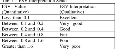
Application of Feature Selective Validation to Propagation Path Loss Models for Wireless Cellular Networks

(1)

Application of Feature Selective Validation to

Propagation Path Loss Models for Wireless

Cellular Networks

Ogundapo Olusegun, Oborkhale Lawrence, Ogunleye Babatunde

The Feature Selective Validation (FSV) algorithm is a technique that allows the quantitative comparison and validation of data.FSV can compare large volumes of complex data and also put the results in a comprehensible form. In this paper, the FSV technique is extended to the comparison and validation of path loss model predictions for wireless cellular networks. The path loss measurements obtained from a base station in the urban area of Yola, Nigeria were compared with predictions made by the COST-231 Hata, Lee and COST-231Walfisch-Ikegami models using the FSV.The results show a Global Difference Measure (GDM) of 0.1403, 0.0922 and 0.1588 for COST-231 Hata, Lee and COST-231 Walfisch-Ikegami path loss models respectively. This indicates that the Lee Model gave a better prediction of the environment making the FSV a useful tool for fast quantitative comparison and validation of standardized path loss model predictions over an environment.

Keywords- Feature Selective Validation, wireless cellular network, propagation path loss models.

I INTRODUCTION

The Feature Selective Validation (FSV) algorithm has been developed to compare two sets of data and put them in an objective form. FSV allows the automated comparison of large volumes of complex data while reliably categorizing the results in a common set of quality band. [1]Propagation models are used extensively in network planning, particularly for conducting feasibility studies and during initial deployment. They are also very useful for performing interference studies as the deployment proceeds and optimization of radio resources. Empirical and semi-empirical propagation models have found favour in both research and industrial communities owing to their limited reliance on detailed knowledge of the terrain.

Manuscript received December 10, 2012, revised February 25, 2013.

All the authors listed above are with the Telecommunications and Wireless Technologies Department, School of Information Technology and Computing, American University of Nigeria, Yola, Nigeria.

Ogundapo Olusegun (e-mail:[email protected]) Oborkhale Lawrence (e-mail:[email protected]) Ogunleye Babatunde (e-mail:[email protected])

However, these models were formulated based on extensive studies and observations in different environment. The effect of radio wave propagation impairments varies from one environment to another.[2] There is the need to have a fast and reliable means of examining the path loss predictions over other environments to minimize errors in their usage. The Feature Selective Validation (FSV) method of validating data will therefore be applied to measured and path loss predictions by the three models under consideration. The study of the path loss prediction behaviour aids effective network planning and optimization of radio resources. The aim of this paper is to apply FSV to the data sets obtained from measurements and predictions by the COST-231 Hata, Lee and COST-231 Walfisch-Ikegami model to determine their suitability for coverage prediction and planning in the area.

The remaining part of the paper is organized as follows: section 2 gives the theoretical basics needed for the research work. Section 3 provides the methodologies used to carry out the research and the results obtained. Section 4 discusses the results of the study. Section 5 concludes the research.

II THEORETICAL BASICS

The two empirical propagation path loss models to be used in this analysis are the COST-231 Hata and Lee models, while the semi-empirical propagation path loss model is that of the COST-231 Walfisch-Ikegami model.

A. COST-231 Hata Model

This is a popular model for predicting the path loss of mobile wireless systems of not more than 10km between the transmitter and receiver. The model was first described by Okumura et.al. and Hata for the prediction of path loss of land mobile radio of not more than 1500 MHz It was later modified by the COST-231 project to include predictions of path loss up to 2000MHz and the provision of correction factors for urban, suburban and rural areas. The basic equation for path loss in dB is: [2][3][4]

 

c

   

bs m

P

f

h

a

h

L



46

.

3



33

.

9

log



13

.

82

log



 





h

b



 

d



C

m



44

.

9

6

.

55

log

(1)

 

h

_m



3

.

2



log



11

.

75

h

_m





2



4

.

97

a

(2)

B. Lee Model

This is another widely used empirical path loss prediction model in mobile wireless systems. It was first described using a base station height of 30.4m, carrier frequency of 900MHz, mobile station height of 3m, maximum distance between transmitter and receiver of 1.6km.Correction factors were then provided that enabled longer distances and other parameters to be included for path loss prediction. The set of equations that define this path loss model are: [5] [6]

                MHz f n km d L c P 900 log 10 6 . 1 log 51 . 30

124



o

(3)

Where,



o





1



2



3



4



5

(4)

 

2 1

48

.

30











m

NewH

_BS



(5)

 

3 2

3











m

NewH

_MS



(6)

 

2 3

10











W

tterPower

NewTransmi



(7)











4

4 A

NewBSG



(8)



5



New mobile station gain (9) Where,

H

BS and

H

MS are the heights of base station and

mobile station respectively in meters,

BSG

_A is the base

station antenna gain in

dBi

and is defined as

3

dB

for

f

_c

>400MHz.

d

is the distance between the transmitter and receiver in meters,

f

c is the carrier frequency in MHz and

o



is the correction factor.

C. COST-231 Walfisch-Ikegami Model.

This is a semi-empirical path loss prediction model for mobile wireless systems of not more than 5km between the transmitter and receiver. The model consists of inputs from publications made by Walfisch et al [7] which provided for the multiscreen diffraction loss and Ikegami et al. [8] that considered an approximation for the roof top to street diffraction loss. The model was later modified by the COST-231 project to include correction factors for antenna heights. It can be used for path loss prediction of mobile wireless systems

up to 2000MHz.The equations that define this path loss model are: [2][3][8]

msd rts o

P

L





(10)

Where

L

o is the path loss due to free space,

L

rts is the

rooftop to street diffraction and scatter loss and

L

msd is

the multi screen diffraction loss.































Km

d

MHz

f

L

o

32

.

44

20

log

c

20

log

(11)

































MHz

f

m

w

L

rts

16

.

9

10

log

10

log

c

roof m

L

_ori

m

h

















log

20

(12)



















km

d

K

L

msd bsh a d

log



























m

b

MHz

f

K

f

log

c

9

log

(13)

Where,

L

_ori is the path loss due to the orientation angle and is defined as:



























































0 0 0 0 0 0

90

55

35

deg

114

.

0

.

4

55

35

deg

075

.

0

5

.

2

35

0

deg

354

.

0

10



ori

L

(14)

d

is the distance between the transmitter and receiver in metres and

f

c is the carrier frequency in MHz b, w and

m

h

are the average buildings separation, average width of street and height of mobile station respectively in metres.

54



a

K

and

K

d



18

.



bs



bsh

h

L





18

log

1





(15)





















1

925

5

.

1

4

c f

f

K

(16)

D. Feature Selective Validation

The Feature Selective Validation technique was selected to compare data from measurement and prediction due to its ability to compare, validate and put them in an objective way. The FSV is therefore an algorithm that has been developed to compare two sets of bidimensional data and put them in an objective and comprehensible form. It is a software that can be found at [10]

(3)

[image:3.595.43.283.239.346.2]

features between the data sets. The GDM is an overall single figure goodness-of-fit between the two data sets being compared. The ADM, FDM and GDM are then compared on a point-by-point basis to give the ADMi, FDMi and GDMi. This allows the user to analyze the resulting data in some detail, probably with the aim of understanding the origin of the contributors to poor comparisons. A lower score means better agreement. The ADMi, FDMi and GDMi can be used to create histogram of the number of points in various agreement categories. These histograms are referred to as ADMC, FDMc and GDMc. The current agreement categories are excellent, very good, good, fair, poor and extremely poor. The FSV interpretation scale is shown in Table 1. [9]

Table 1: FSV Interpretation Scale FSV Value

(Quantitative)

FSV Interpretation (Qualitative) Less than 0.1 Excellent Between 0.1 and 0.2 Very good Between 0.2 and 0.4 Good Between 0.4 and 0.8 Fair Between 0.8 and 1.6 Poor Greater than 1.6 Very poor

III IMPLEMENTATION AND RESULTS

The signal strength measurement was carried out in the urban area of Yola, Nigeria. The area consists of buildings whose average height is about seven floors (24m). The signal strength measurements were collected through drive tests with the aid of Ericsson Test Mobile System (TEMS) along the open route of the wireless mobile network base station. The TEMS was connected to a laptop with the aid of a Global Positioning System (GPS) for tracking the distance between the base station and the mobile station. The height of the receiver was about 1.5m.The Path loss for each base station was computed using the COST-231 Hata, Lee and COST-231 Walfisch- Ikegami Path loss models. The FSV software was then used to compare the measurements and predictions made by the models.

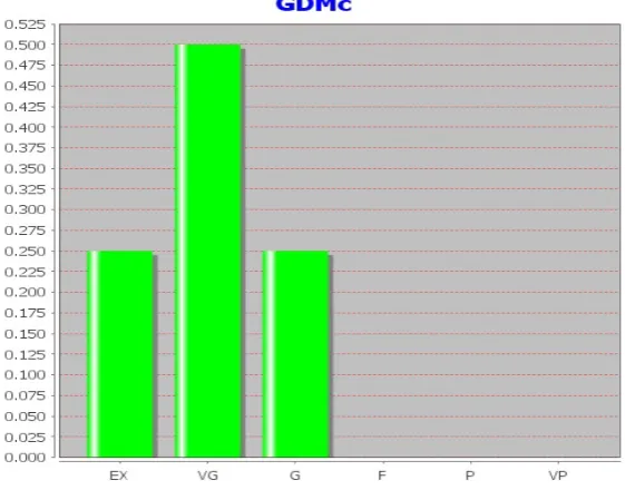
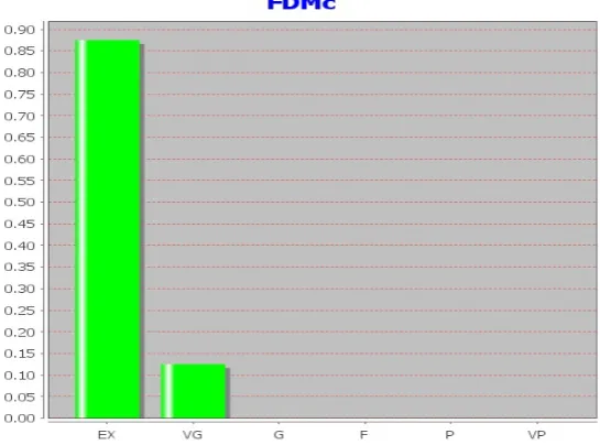
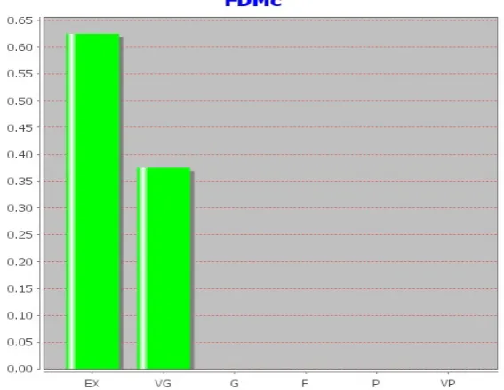
The FSV comparison of the three models with measurement presented in histogram forms are shown in Figures 1 to 9. The summary of the ADMc, FDMc and GDMc results are shown in Table 2.

Table 2: FSV Summary Values Total

Values

Hata Lee Walfisch

ADMc 0.1360 0.1139 0.1470 FDMc 0.0695 0.0557 0.0855 GDMc 0.1403 0.0922 0.1588

IV DISCUSSIONS OF RESULTS

The plots in Figures 1 to 9 shows the ADMc, FDMc and GDMc results presented in histogram form for the comparison between measured and COST-231 Hata, Lee and COST-231 Walfisch-Ikegami models using the FSV software. The GDMc results which is a combination of

the ADMc and the FDMc indicates that the Lee model gave a better prediction of the environment as shown in Table 2. This is corroborated by the GDMc plot for the comparison between measurement and the Lee model in Figure 6 which has most of the comparison results within the excellent range than the COST-231 Hata and Walfisch-Ikegami models. The summary of quantitative values from the ADMc, FDMc and GDMc comparisons are presented in Table 2.

V CONCLUSION

This paper presents the application of the FSV tool to compare measurement and path loss predictions using the COST-231 Hata, Lee and COST-231Walfisch-Ikegami models. The result show that the Lee model has a GDMc of 0.0922 which indicates a better prediction of the environment than the 0.1403 and 0.1588 provided by the COST-231Hata and COST-231 Walfisch-Ikegami models respectively. The FSV tool therefore provided a faster quantitative comparison and validation of standardized propagation path loss model predictions for the environment.

Reference

[1]. V.Rajamani et al, “Introduction to Feature Selective Validation (FSV)’’, in the proceeding of the International Symposium on Antennas and Propa-gation Society,pp.601-604,2006.

[2]. COST 231, “Digital Mobile Radio Towards Future Generation Systems’’, COST 231 Final Report, Ch 4, pp.134-140.

[3]. J.S Seybold, “Introduction to Radio Frequency Propagation’’, published by John Wiley and Sons, pp.152-153.

[4]. J.D Parsons, “The Mobile Radio Propagation Channel’’,2nd ed.,published by John Wiley, West Sussex, 2000,pp.85-86.

[5]. N.Blaunstein, Radio Propagation in Cellular Networks, Artech House Norwood, MA, 2000, pp.275-279.

[6]. W.C.Y Lee, Mobile Communication Design Fundamentals, 2nd ed., John Wiley, New York, 1993, pp.59-67.

[7]. J. Walfisch et al. “A Theoretical Model of UHF Propagation in Urban Environments”, IEEE Transaction on Antenna and Propagation, Vol. 36, No. 12, pp.1788-1796, 1988.

[8]. F. Ikegami et al “Propagation Factors controlling Mean Field Strength on Urban street” IEEE Transactions on Antenna Propagation, Vol. 32, pp. 822- 829, 1984.

[9]. Duffy, A. Martin, et al. “The Feature Selective Validation (FSV) Method”, in proceedings of the IEEE Symposium on Electromagnetic Compatibility, Chicago, USA, Vol.1, pp.272-277, 2005.

[10]. FSV_Tool_2_0L Tool:

(4)

[image:4.595.51.333.55.233.2] [image:4.595.52.333.270.472.2]

Figure 1: ADMc Results for Measured and Hata Model Comparison

Figure 2: FDMc Results for Measured and Hata Model Comparison

[image:4.595.52.333.498.718.2]

(5)

[image:5.595.51.325.54.280.2]

Figure 4: ADMc Results for Measured and Lee Model Comparison

[image:5.595.52.325.322.524.2]

Figure 5: FDMc Results for Measured and Lee Model Comparison

[image:5.595.56.329.565.751.2]