Abstract— This paper proposes a new structure of heating feed-forward control system for multi-storey buildings based on indoor air temperature inverse dynamics model. The suggested model enables real-time assessment of the impact of perturbing factors that cannot be directly measured on indoor air temperature with due allowance for lag and nonlinear nature of thermohydraulic processes involved in the building heating cycle. To measure current indoor air temperature values, the authors used a distributed field-level sensor network. This paper contains the results of identification for the formulated model, as well as a calculation of energy savings after deployment of heating control system in the academic building of South Ural State University in accordance with International Performance Measurement and Verification Protocol (IPMVP).
Index Terms— Building thermal performance simulation, feed-forward control, inverse dynamics model, heating of buildings, automated heat station
I. INTRODUCTION
AKING building heating systems more efficient is one of the key tasks of energy and resource conservation. In Russia and some other northern countries, where heating season takes up most of the year, heating costs account for the majority of spendings on energy resources consumed by residential and office buildings. For example, the share of heating energy in overall energy consumption of South Ural State University main campus totals 36.7%, which ultimately corresponds to 30,100 Gcal (based on the 2012 energy audit).
Energy efficiency of heating systems used in buildings could not possibly be upgraded without automatic control systems that implement a variety of control algorithms [1]– [3]. Baseline control principle used in these systems is control of the indoor temperature by reference to the primary perturbing factor, i.e. outdoor temperature Tout. This approach appears viable, as it guarantees adequate quality, while implementing simple control algorithms and using
Manuscript received July 23, 2014; revised July 29, 2014.
D. A. Shnayder is with the Automatics and Control Department, South Ural State University, Chelyabinsk, Russia (phone: +7-351-751-1212; e-mail: [email protected]).
V. V. Abdullin is with the Automatics and Control Department, South Ural State University, Chelyabinsk, Russia (corresponding author to provide phone: +7-351-777-5667; fax: +7-351-267-9369; e-mail: [email protected]).
A. A. Basalaev is with the Automatics and Control Department, South Ural State University, Chelyabinsk, Russia (phone: +7-912-772-2514; e-mail: [email protected]).
data that is easy to measure. However, the key factor that determines the quality of heating system performance is indoor air temperature Tind. This is why it is important to design heating control systems that take into account the actual Tind values. Control principle based on Tind is described in a number of papers [4]–[5], but there are certain challenges that make practical implementation of this approach rather problematic:
– air temperature varies in different rooms of a multi-storey building;
– building heating system is highly inertial and performs as a nonlinear distributed system, which renders control by indoor air temperature rather difficult in a situation when common engineering methods are employed;
– the building is exposed to numerous perturbing factors (Fig. 1) that are hard to measure or evaluate in real terms.
The indoor air temperature Тind of a building depends on its volume, building envelope type, the quantity of applied heating energy Qsource, inner and external perturbing factors, such as the outdoor air temperature Тout, solar radiation Jrad, wind Vwind, internal heat release Qint, and the building’s accumulated internal heating energy Qacc [8]. However, the signals Тind, Qsource, and Тout presented in Fig. 2 can be measured quite easily in practice, while direct measurement of Jrad, Vwind, Qint, and Qacc that affect the temperature Тind is actually problematic.
These are the reasons why most heating control systems for multi-storey buildings that exist on the market and are widely deployed in real life either completely disregard the indoor air temperature, or refer to its value only to monitor the quality of control measures, without actually using it to adjust the control signal.
To solve above-mentioned problems, complex objects of this sort are now commonly designed in accordance with model-predictive control methods [6]–[7] that are based on mathematical modeling of the object. This paper describes a new approach to heating control in a multi-storey building that is based on estimation of perturbations affecting on the
Building Heating Feed-forward Control
Based on Indoor Air Temperature
Inverse Dynamics Model
Dmitry A. Shnayder, Vildan V. Abdullin, and Aleksandr A. Basalaev
M
Building Tout
Jrad Vwind
Qsource Tind
Qint
[image:1.595.312.530.678.774.2]Qacc
indoor air temperature using the building thermal performance inverse dynamics model.
II. CONTROL APPROACH BASED ON INVERSE DYNAMICS MODEL
A. Feed-forward control system structure
To take into account the unmeasured factors that affect temperature Тind(t), we referred to the approach based on the concept of generalized temperature perturbation Tz(t) [8] characterizing the effect of the factors mentioned above on the indoor air temperature.
Generic structure of the proposed feed-forward control system is described in Fig. 2. As we see in the figure, baseline control of heat supply for building heating purposes follows a standard pattern with the use of automated building heat station that controls heating power QhTout depending on the key perturbing factor – outdoor air temperature. The structure shown in Fig. 1 is augmented by a feed-forward control loop used to adjust QhTout depending on estimated value Т’z of general temperature perturbation
Тz. Thus, the adjusted heating power value QhTind fed into the building is calculated as follows:
ind out ind,
T T T
h h h
Q Q Q (1)
where ΔQhTind – adjusting value of heating power produced by feed-forward temperature controller.
Let us consider the inverse dynamics model. In accordance with [8], the heat balance equation takes the following form:
h
ind ind z
h
,
Q t
T t T t T t
q V
(2)
where T’ind(t) stands for the predicted value of indoor air temperature (the prediction horizon is determined by the fluctuation of indoor air temperature as a result of the perturbing factors (Fig. 1)); Tout(t) is outdoor air temperature; Qh(t) stands for heating power applied to the heating system from the heating radiator; qh represents specific heat loss (per cubic meter); and V stands for external volume of the building.
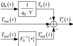
A block diagram of building thermal performance dynamics model composed in accordance with (2) is presented in Fig. 3. The key input signal in this model is represented by heating power Qh(t) delivered by heating radiators and generated by the heat station. The dynamics operator F0{•} describes building’s heat exchange process dynamics [8].
According to the model shown in Fig. 3, the feed-forward value of indoor air temperature can be determined by the following equation:
1
ind 0 ind ,
T t F T t (3)
where F0–1{•} stands for the inverse dynamics operator calculated using the exponential filtration method [8]–[9]. Consequently, the estimated value of general temperature perturbation T’z can be counted as follows:
h 1
z out 0 ind
h
,
Q t
T t T t F T t
q V
(4)
that is presented on Fig. 4.
The main difference of this approach from other works like [10] is that this is an out-of-the-box solution that includes a way to estimate disturbances.
B. Modeling thermohydraulic performance of the building’s heat station
In addition to building heat exchange processes, the structure and performance of equipment installed in the building’s heat station have a significant impact on the heating process. In this regard, let us review the model of thermohydraulic performance of the building’s heat station.
Heat station is a fairly complex engineering facility. It contains control devices (valves, pumps) with nonlinear properties, as well as process controllers that implement certain control algorithms (typically, a PID controller with control signal depending on outdoor air temperature in accordance with heating curve). A heat station of this sort is deployed in the academic building1, which was used for the research.
Heat station of the studied building has a standard design with a pump group on the supply pipeline, control valve on the return pipeline, and a displacement bypass with a check valve to prevent direct flow from supply pipe to return pipe. The building’s heating system has a vertical design with down-feed risers and single-pipe radiator connections.
1
Ten-storey academic building of South Ural State University at the following address: Bldg. 3BV, 87 Lenina prospekt, Chelyabinsk, 454080, Russia. External volume: 71,573 m3.
Building Heat Station
ind
T h
Q Building
Heating System
z
T
ind
T
Inverse Dynamics
Model Feed-forward
Temperature Controller
z
T
out
T
ind
T h
Q
out
T h
Q
out
T
out
[image:2.595.315.539.405.526.2]T
Fig. 2. Generic structure of the building heating control system with feed-forward temperature controller.
h 1
q V F0
•
hQ t
outT t
zT t
hT t Tind
t Tind
tFig. 3. Block diagram of the building thermal performance dynamics model.
outT t T tz
hT t
indT t
h 1
q V
1 0 •F
indT t
hQ t
[image:2.595.323.535.573.622.2] [image:2.595.365.490.660.738.2]The model represents thermohydraulic processes modelled in VisSim visual modeling software on the basis of the model proposed in [11]. The model provides numerical solution of a system of algebraic equations that describe hydraulic processes in the heat medium and transfer of heating energy between the heat medium and heat load. For convenience, the model is represented as an array of independent functional blocks that describe standard elements of the heating system: pipe, control valve, check valve, pump, heat load, etc. Each functional block contains all the equations that describe the processes inherent to the block with a desired approximation. The blocks are tied by unidirectional connections, and the direction of connection corresponds to the positive direction of flow (flow rate
G > 0). Each connection is a vector of three elements, including absolute pressure P [Pa], mass flow rate G [kg/s], and temperature T [°C], which characterizes parameters of heat medium in the corresponding pipe section. Therefore, connections between the blocks can be associated with physical connection of elements.
The key input signal in this model is the position of stem in control valve Y, 0…1, assigned by the process controller
installed in the heat station. The model’s output value is heating power Qh emitted into the rooms of the building by heating radiators.
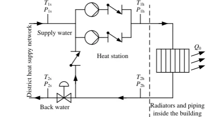
The simplified Piping and instrumentation diagram (P&ID) of heat station and building’s heating system is shown in Fig. 5. The set of static response curves for this model is shown in Fig. 6. As we can see from the figure, this is a nonlinear model.
The model includes distributed elements (pipelines and heating radiators). The entire path of heat medium from the the distributed element’s point of inlet up to the point of exit from such element (from 0 to L, where L is the length of heat medium path) is decomposed into N sections, each having the length of dx. Water temperature inside each
section is assumed to be invariable and equals T(x). This helps us simulate the transportation lag determined by the final rate of heat medium movement inside the pipeline.
Models of key functional blocks built in accordance with the above approach are described in the text below.
Heating feed
For the heating feed, the values of pressure in the supply and return pipelines (P1s and P2s, respectively) and supply water temperature T1s are known. These parameters are independent of the hydraulic parameters of the circuit connected to the heating feed. This is why we selected flow rate of heat medium from heating network G1s as the unknown parameter, and pressure error in the return pipeline – as the solution criterion. Therefore, heating feed includes an unknown variable and a condition that jointly make up the following equation:
2 back 1s, 1s 2s 0 ,
P G P P (5)
where function P2 back ( G1s, P1s ) stands for pressure of returned heat medium calculated on the basis of structure of hydraulic network connected to the heating feed.
On a VisSim model diagram, heating feed block has one output that corresponds to the supply pipeline and one input that corresponds to the return pipeline.
Control valve
In general, head loss in any hydraulic section is determined in accordance with the following formula:
2 sign ,
P G G s
(6)
where ΔP is delta pressure at input and output of the section,
G – mass flow rate of heat medium, and s – fluid resistance. Multiplication factor signG is used to account for possible change in flow direction.
The fluid resistance in open and closed positions sopen and
sclose is employed to model the valve’s rate of opening. Actual value of fluid resistance of the valve sv is determined in accordance with the following rule:
v v open close close ,
s f Y s s s (7)
where Y = 0…1 is the valve’s rate of opening, and function
fv(Y) determines the valve’s regulating performance (fluid resistance to stem position behavior). Control valve is presumed to have no heat loss, meaning that heat medium output temperature equals its input temperature. Therefore, control valve’s performance can be described by the following equations:
2
v out v in v v v open close close
v out v in v
v out v in
sign ;
;
,
P P G G f Y s s s
G G G
T T
(8)
where Pv in, Pv out, Gv in, Gv out, Tv in, Tv out stand for the values of heat medium pressure, flow rate and temperature at the input and the output of the control valve respectively.
Check valve
In general, check valve resistance scv drops when flow
T1s
T2s P1s
P2s
T1h
T2h P1h
P2h
Heat station
Radiators and piping inside the building
D
is
tr
ic
t
h
ea
t
su
p
p
y
n
et
w
o
rk
Supply water
Back water
[image:3.595.49.273.471.761.2]Q0
Fig. 5. Simplified P&ID of the building’s heat station.
Fig. 6. Set of static response curves for heat station model.
[image:3.595.52.261.490.607.2]rate Gcv grows, and it rises steeply when Gcv drops below zero. As in the case with control valve, check valve is presumed to have no heat loss. Therefore, check valve can be described by the following equations:
2
cv out cv in cv cv cv cv
cv out cv in cv
cv out cv in
sign ;
; ,
P P G G s G
G G G
T T
(9)
where Pcv in, Pcv out, Gcv in, Gcv out, Tcv in, Tcv out stand for the values of heat medium pressure, flow rate and temperature at the input and the output of the check valve respectively.
Pump
Differential pressure between the pump’s input and output ΔPp is described by a nonlinear function:
p p p ,
P f G
(10)
where Gp is the flow rate of heat medium pumped, and function fp(Gp) describes the pump’s parameter specified in the pump data sheet.
As in the case with control valve, pump is presumed to have no heat loss. Therefore, pump can be described by the following equations:
p out p in p p
p out p in p
p out p in
;
;
,
P P f G
G G G
T T
(11)
where Pp in, Pp out, Gp in, Gp out, Tp in, Tp out stand for the values of heat medium pressure, flow rate and temperature at the input and the output of the pump respectively.
Radiator equivalent
Each elementary volume of water contained in the dx
section of heating radiator at any given point in time is involved in heat exchange with the environment. This heat exchange process is described by the following equation:
h h h h ind h
dT k W T x T dx c G (12)
where dTh is the variation of temperature of elementary heat medium volume, kh [ W/(m2∙°C) ] – heat transfer ratio,
Wh = Sh / Lh – width of heat medium path, Sh – radiator transfer section area, Th(x) – function of temperature distribution along the path of heat medium, с – heat capacity of water, and Gh – heat medium flow rate.
The result is a differential equation that describes distribution of heat medium temperature inside the radiator:
h h h h ind h
dT dx k W T x T c G (13)
When solved, the equation results in the following relation:
h h h
h ind h in h out
k W x c G
T x T T T e (14)
Water temperature at radiator output Th out can be determined by replacing x by path length L in (14). Furthermore, any radiator may have its own fluid resistance
sh that leads to head loss (see check valve). Therefore, a heating radiator can be described as:
h h h
2
h out h in h h h h
h out h in h
h out ind h in h out
sign ;
;
,
k S c G
P P G G s G
G G G
T T T T e
(15)
where Ph in, Ph out, Gh in, Gh out, Th in, Th out stand for the values of heat medium pressure, flow rate and temperature at the input and the output of the radiator respectively.
III. APPLICATION OF PROPOSED HEATING CONTROL SOLUTIONS FOR SOUTH URAL STATE UNIVERSITY ACADEMIC
BUILDING
A. Approach to measuring indoor air temperature inside the building based on field-level sensor network
Theoretical studies and experiments show that air temperature in different spaces of the same building may vary significantly as a result of exposure to various perturbing factors described above. This is why building heating control based on indoor air temperature in a single reference area proved to be practically unviable [12]. To solve this problem, we deployed a distributed network of sensors measuring temperature in different premises of the building. The first step was to install 24 digital temperature sensors Dallas 18B20 in different rooms of the academic building linked together in MicroLan (1-wire) network [13]. To simplify the system, we do not measure temperature in windowless premises, such as restrooms, technical areas and unheated hallways. In addition, we conducted an experimental study of wireless data transfer from sensors to
RFM XDM2510HP embedded communication modules
integrated into a WirelessHART wireless sensor network [14]. This technology showed its viability during the case study and will be used in our further research on the subject matter of this study.
The indoor air temperature Тind of a building, which is the average value of indoor temperatures in each room, accounting for differences in area, is calculated as follows:
ind i ind i i ,
i i
T t S T t S
(16)
where Si, Tind i stand for the area and temperature of the i-th room, respectively, and t is time. Using the average temperature Tind permits us to estimate relatively fast perturbations, such as wind, solar radiation, or local heat sources, which affect thermal performance of some rooms, e.g., the rooms of one side of the building – for the entire building.
B. Identification of model parameters based on academic building data
were obtained during the identification process:
– time constant of the building thermal performance model Tbld = 20 hours;
– net lag of building heat performance model τbld = 1 hour;
– average specific heat loss of the building
qh = 0.09 W/(m3∙°C).
Parameters of the control valve and pumps installed in the heat station were defined using original datasheets. Pipeline lengths and diameters used in heat station model are based on the data specified in design and operating documents for the building heating system.
Feed-forward temperature controller was implemented as a PID controller with gains: Kp = 0.1, Ki = 1/9000, Kd = 0.
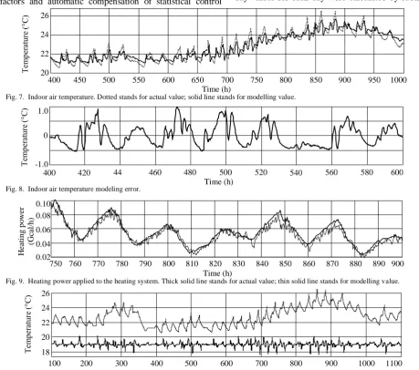
Verification of the resulting model revealed modeling error for indoor air temperature in the range of ±1°C, and the value of root mean square modeling error (RMSE) is 0.263°C. Indoor air temperature chart is shown in Fig. 7, and air temperature modeling error is presented in Fig. 8.
The value of mean absolute percentage error (MAPE) for heating power Qh is 5.7%. The chart of heating power applied to the heating system is shown in Fig. 9.
Energy saving effect of the proposed approach is in the stable control of indoor air temperature at a comfort level, along with a significant reduction of impact of perturbing factors and automatic compensation of statistical control
error caused either by inaccuracy of temperature chart, or by the effects of structural changes in the building’s thermal performance. Fig. 10 shows a chart of actual indoor air temperature fluctuations for the baseline control option and the expected reduction of fluctuations after deployment of feed-forward control.
C. Savings determination
Below is the analysis of system deployment benefit based on the International Performance Measurement and Verification Protocol (IPMVP).
Stage 1
The first stage of the building’s heating system automation process was intended to deploy a standard automatic control system that adjusts consumption of heat medium depending on the outdoor air temperature (baseline control).
According to IPMVP, a statistical model is required to benchmark system efficiency before and after completion of energy conservation measures (ECM) in the reporting period under comparable conditions.
A linear regression model is used to build the statistical model for the reporting period. The model’s factors include daily values of degree-days, water consumption, and heat medium average temperature at building inlet. The degree-day values for each degree-day were calculated by subtracting the
Fig. 7. Indoor air temperature. Dotted stands for actual value; solid line stands for modelling value.
[image:5.595.47.507.357.763.2]Fig. 8. Indoor air temperature modeling error.
Fig. 9. Heating power applied to the heating system. Thick solid line stands for actual value; thin solid line stands for modelling value.
Fig. 10. Indoor air temperature. Thin solid line stands for actual value in case of control by outdoor temperature; thick solid line stands for expected value in case of feed-forward control deployment.
Time (h)
400 450 500 550 600 650 700 750 800 850 900 950 1000
T
em
pe
ra
tur
e
(°
C
)
20 22 24 26
Time (h)
T
em
pe
ra
tur
e
(°
C
)
400 420 44
0
460 480 500 520 540 560 580 600
-1.0 0 1.0
Time (h)
H
ea
ti
ng
po
w
er
(G
ca
l/
h)
750 760 770 780 790 800 810 820 830 840 850 860 870 880 890 900 0.02
0.04 0.06 0.08 0.10
Time (h)
T
em
pe
ra
tur
e
(°
C
)
100 200 300 400 500 600 700 800 900 1000 1100
values of outdoor air temperature specified in the archives of local weather station from the nominal value of indoor temperature (20°C). Water consumption and heat medium average temperature values were measured by the building’s meters on a daily basis.
The baseline period was determined as the period from March 20, 2013 until April 17, 2013, which corresponds to the reporting period from March 20, 2014 until April 17, 2014. March 20 is the date of ECM completion and system commissioning in 2014. April 17 is the end date of the heating season in 2013, which ended earlier than in 2014.
The optimal regression values for the heating season were obtained if only one factor is used (daily degree-days Dd). Daily heat energy consumption Ed is calculated in the regression model as follows:
d 1 d ,
E a D (17)
where a1 = 0.43 is a degree-day regression parameter as a
result of the linear regression analysis.
For the period under consideration, the coefficient of determination R2 in the linear regression model equals 0.97 with confidence level of 0.95 (n1=28 days). The value is higher than 0.75, that proves high statistical significance of the model in accordance with IPMVP. The degree-days factor passes the Student’s t-test (t1 = 2.06 < testim = 28.96), and the P-value (P = 7∙10–22) is much lower than the significance point of 0.05, which indicates high statistical significance of this factor.
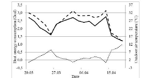
Then adjusted-baseline heat energy consumption was calculated for the reporting period using (17). Fig. 10 represents heat energy consumption in the baseline period. Fig. 11 represents actual heat energy consumption and adjusted-baseline heat energy consumption in the reporting period.
Standard error of daily heat energy consumption in the model is as follows: SE1=1.65 Gcal. Standard error of adjusted-baseline heat energy consumption for the entire baseline period SEABL1 is calculated using the following formula [15]:
2
ABL1 1 .
SE n SE (18)
Calculated standard error for the entire reporting period is 8.72 Gcal.
Absolute error of heat energy consumption for the entire period AEABL1 in the model with account for the t-value (t1=2.06) is calculated using the following formula:
ABL1 ABL1 .
AE SE t (19)
Calculated absolute error for the entire reporting period is 17.93 Gcal.
Estimated adjusted-baseline heat energy consumption in the reporting period E*ABL1 under comparable conditions without account for the error is 234.06 Gcal. Actual value of consumed heat energy ERP1 is 162.14 Gcal. The value of savings E*ECO1 without account for error is E*ECO1 = = E*ABL1 – ERP1 = 71.92 Gcal.
The value of savings without account for error in the reporting period is more than four times higher than the standard error. This meets the condition of acceptable uncertainty. According to IPMVP [15], savings must be at least twice higher than standard error.
Thus, savings EECO1 with account for error AEABL1 total 71.92±17.93 Gcal.
The value of minimum relative savings with account for error AEABL1 is calculated using the following formula:
*
min ABL1 ABL1 RP1
REL ECO1 *
ABL1 ABL1
( )
100%.
E AE E
E
E AE
(20)
Minimum relative savings in the reporting period total 25.0%.
Stage 2
Stage 2 is intended for practical deployment of feed-forward control approach proposed in this study based on the reverse dynamics model.
Source model of baseline consumption was calibrated in
Fig. 11. Heat energy consumption in the baseline period. Dotted line stands for outdoor air temperature; dashed line stands for heat energy consumption.
Fig. 12. Benchmarking of adjusted-baseline and reporting-period heat energy consumption in the reporting period. Dotted line stands for outdoor air temperature; dashed line stands for actual heat energy consumption; solid line stands for adjusted-baseline heat energy consumption.
Fig. 13. Benchmarking of heat energy consumption before and after ECM under comparable conditions. Dashed line stands for baseline heat energy consumption before ECM; solid line stands for chart of heat energy consumption after ECM; dotted line stands for outdoor air temperature chart.
-15 5 25 45 -5 0 5 10 15
20.03 30.03 08.04 17.04
O ut do o r a ir te m pe ra tur e, ° C H ea t en er gy co n sum pt io n , G ca l Date -15 -5 5 15 25 35 45 55 -5 0 5 10 15
20.03 30.03 08.04 17.04
O ut do o r a ir te m pe ra tur e, ° C H ea t en er gy co n sum pt io n , G ca l Date -15 -5 5 15 25 35 45 55 -5 0 5 10 15
20.03 30.03 08.04 17.04
[image:6.595.48.280.290.408.2] [image:6.595.44.282.449.573.2] [image:6.595.44.285.620.746.2]accordance with the building’s heat meters in the period from March 20, 2014 until April 17, 2014, which corresponded to the reporting period of the previous stage. The model for the upgraded system was built by introducing a feedback control module.
Fig. 13 represents modeling results for one month of the heating season.
Model calibration standard error of hourly heat energy consumption after outlier filtering is as follows:
SE2 = 0.007 Gcal. Model calibration standard error for the entire period SEC is calculated using the following formula:
2
C 2 2,
SE n SE (21)
where n2 is a sample size (n2 is 501 after outlier filtering). Calculated standard error of model calibration for the entire period is 0.16 Gcal.
Model calibration absolute error for the entire period AEC with account for the t-value (t2=1.97) is calculated using the following formula:
C C 2.
AE SE t (22)
Calculated absolute error of model calibration for the entire period AEC is 0.32 Gcal.
Total heat energy consumption is calculated after model calibration and outlier filtering. Estimated total baseline heat energy consumption E*BL2 without account for error is 54.08 Gcal. Estimated total report-period heat energy consumption
E*RP2 without account for error is 48.15 Gcal.
The value of minimum relative savings with account for error AEC is calculated using the following formula:
* max * max
min BL2 C RP2 C
REL ECO2 * max
BL2 C
* * * max
BL2 RP2 BL2 C
( ) ( )
100%
100% .
E AE E AE
E
E AE
E E E AE
(23)
Thus, based on the modeling results, additional relative savings from practical deployment of the authors’ proposed approach were estimated at 10.9%.
IV. CONCLUSION
The results obtained demonstrate the overall viability of the proposed approach that accounts for the indoor air temperature and employs feed-forward control based on thermal performance inverse dynamics model, as well as prove high efficiency of this approach in automatic heating control systems. If deployment of baseline control by outdoor air temperature showed in practice a minimum 25.0% saving of heating energy, according to the simulation results it is expected to obtain about 10% extra saving of heating energy in case of deploying the proposed feed-forward control.
Deployment and experimental studies of the proposed heating feed-forward control will be completed in hardware in the studied academic building of South Ural State University in the next heating season starting in October 2014.
ACKNOWLEDGMENT
V. V. Abdullin expresses his deep appreciation to Mikhail V. Shishkin for the technical advices on heating station equipment modelling.
REFERENCES
[1] Y. A. Tabunschikov, M. M. Brodach, Mathematical modeling and
optimization of building thermal efficiency, (Russian:
Математическое моделирование и оптимизация тепловой эффективности зданий.) – Moscow: AVOK-PRESS, 2002. [2] J. M. Salmerón, S. Álvarez, J. L. Molina, A. Ruiz, F. J. Sánchez,
“Tightening the energy consumptions of buildings depending on their typology and on Climate Severity Indexes,” Energy and Buildings, vol. 58, 2013, pp. 372–377.
[3] D. Zhou, S. H. Park, “Simulation-Assisted Management and Control Over Building Energy Efficiency – A Case Study”, Energy Procedia, vol. 14, 2012, pp. 592–600.
[4] D. A. Shnayder, M. V. Shishkin, “Adaptive controller for building heating systems applying artificial neural network” (Russian: Адаптивный регулятор отопления здания на основе искусственных нейронных сетей), Automatics and control in technical systems, Edited book – Chelyabinsk: South Ural State University press, 2000, pp. 131–134.
[5] P.-D. Moroşan, “A distributed MPC strategy based on Benders’ decomposition applied to multi-source multi-zone temperature regulation,” Journal of Process Control, vol. 21, 2011, pp. 729–737. [6] T. Salsbury, P. Mhaskar, S. J. Qin, “Predictive control methods to
improve energy efficiency and reduce demand in buildings”, Computers and Chemical Engineering, vol. 51, 2013, pp. 77–85. [7] E. Žáčeková, S. Prívara, Z. Váňa, “Model predictive control relevant
identification using partial least squares for building modeling,” Proceedings of the 2011 Australian Control Conference, AUCC 2011, Article number 6114301, pp. 422–427.
[8] V. V. Abdullin, D. A. Shnayder, L. S. Kazarinov, “Method of Building Thermal Performance Identification Based on Exponential Filtration,” Lecture Notes in Engineering and Computer Science: Proceedings of The World Congress on Engineering 2013, WCE 2013, 3–5 July, 2013, London, U.K., pp. 2226–2230.
[9] L. S. Kazarinov, S. I. Gorelik, “Predicting random oscillatory processes by exponential smoothing” (Russian: Прогнозирование случайных колебательных процессов на основе метода экспоненциального сглаживания), Avtomatika i telemekhanika, vol. 10, 1994, pp. 27–34.
[10] B. Thomasa, M. Soleimani-Mohsenib, P. Fahlén, “Feed-forward in temperature control of buildings”, Energy and Buildings, vol. 37, 2005, pp. 755–761.
[11] M. V. Shishkin, D. A. Shnayder, “Modelling thermo-hydraulic processes using Vissim simulation environment” (Russian: Моделирование теплогидравлических систем в среде VisSim), Bulletin of the South Ural State University, Series Computer Technologies, Automatic Control, Radio Electronics, vol. 3., 9 (38) 2004, pp. 120–123.
[12] S. V. Panfyorov, “Adaptive control system of building thermal conditions” (Russian: Адаптивная система управления тепловым режимом зданий), Proceedings of the 7th Russian national scientific and engineering conference ‘Automatic systems for research, education and industry’ – Novokuznetsk, 2009, pp. 224-228. [13] M. V. Shishkin, D. A. Shnayder, “Automated process monitoring and
control (SCADA) system based on MicroLan” (Russian: Автоматизированная система мониторинга и управления технологическими процессами на основе сети MicroLan), New software for business of Ural region, Issue 1, Proceedings of the regional scientific and engineering conference – Magnitogorsk: Magnitogorsk State Technical University press, 2002, pp. 84–89. [14] D. A. Shnayder, V. V. Abdullin, “A WSN-based system for heat
allocating in multiflat buildings,” 2013 36th International Conference on Telecommunications and Signal Processing Proceedings, TSP 2013, 2-4 July, 2013, Rome, Italy, Article number 6613915, pp. 181– 185.