Multi-Scale Subspace Grids Based Approach for Recognising Patterns in Applications Involving Multidimensional Data

(1)

Multi-Scale Subspace Grids Based Approach for

Recognising Patterns in Applications Involving

Multidimensional Data

M. Arif Wani

Abstract—The work presented in this paper employs multi-scale subspace grids for pattern recognition applications. The proposed approach addresses the curse of dimensionality problem often associated with this task. The paper uses a multi-scale approach where coarse scale, being stable and generic in nature, suits well for small sample sizes, and fine scales, being more specialized in nature, enhance classification accuracy. The paper first describes projection of multidimensional data to a number of lower dimensional subspaces. Principal component analysis (PCA) and multiple discriminant analysis (MDA) algorithms are used to define lower dimensional subspaces. The range of value associated with each vector of a subspace is divided into a number of equal parts to define coarse subspace grids. Coarse subspace grids are further divided equally into fine subspace grids. The approach is tested on two applications. In first application, a recursive procedure is employed to obtain rules from multi-scale subspace grids to recognize patterns. In second application, a neural network algorithm is used to recognize patterns using multi-scale subspace grids. The results show that the use of subspaces grids produces good results to recognize patterns in multidimensional data.

Keywords—subspace grids; machine learning; pattern recognition; principle component analysis; multiple discriminant analysis; multi-scale approach.

I. INTRODUCTION

Recognition of patterns in applications involving multidimensional data is one of the important research areas. Curse of dimensionality is normally addressed by projecting multidimensional data to a lower dimensional space. Thus one of the major tasks in analyzing patterns in multidimensional data, associated with a given application, is to project the data to a lower dimensional space first and then analyzing the data in lower dimensional space. This paper employs multi-scale subspace grids in lower dimensional space to recognize pattern. The approach is tested on two data sets: Iris data and data set having features extracted from veneers of wood.

Iris data set is only a four dimensional data set while as wood features data set is a seventeen dimensional data set. Iris data set is a four class problem while as wood features data set is a thirteen class problem. The thirteen classes in wood features data set include twelve defects which are (i) bark (ii) coloured streaks (iii) curly grain (iv) discoloration (v) holes (vi) pin knots (vii) rotten knots (viii) roughness (ix) sound knots (x) splits (xi) streaks (xii) worm holes. The

M. Arif Wani is with the Computer Science Department, University of Kashmir, Hazratbal, Srinagar, India 190006, and on leave from the Computer and Electrical Engineering and Computer Science Department at California State University Bakersfield, California, CA 93311 (e-mail: [email protected]).

last class is the clear veneer. A literature review of the related work of analyzing multidimensional data is presented in the next section.

II.

L

ITERATURE

R

EVIEW

A lot of literature is available on classification of multidimensional data. Some of the work is summarized in this section.

A comparative study of pattern selection methods for classification of multidimensional data is presented by Chai and Domeniconi [1]. The authors compare several feature ranking techniques, including variants of correlation coefficients, and Support Vector Machine (SVM) method based on Recursive Feature Elimination (RFE). A study by Hori et al. [2] shows that an independent component analysis (ICA) based method can effectively and blindly classify a vast amount of multidimensional data. Based on the results, authors suggest that the ICA based method can be a powerful approach for classification tasks. The authors also examine classification by principal component analysis (PCA), and compare results of PCA and ICA methods.

Pique-Regil et al. [3] propose a sequential Diagonal Linear Discriminant Analysis (SeqDLDA) technique that combines gene selection and classification. At each iteration, one gene is sequentially added and the linear discriminate (LD) recomputed using the SeqDLDA model. Classical Diagonal Linear Discriminant Analysis (DLDA) will add the gene with highest t-test score without checking the resulting model. In contrast, SeqDLDA will find the one gene that better improves class separation after recomputing the model parameters using a robust t-test score. A data-dependent kernel for microarray data classification was presented by Xiong et al. [4]. This kernel function is engineered so that the class reparability of the training data is maximized. A bootstrapping-based resampling scheme is introduced to reduce the possible training bias.

Wang et al. [5] use a hybrid huberized support vector machine (HHSVM). The HHSVM uses the huberized hinge loss function to measure misclassification and the elastic-net penalty to control the complexity of the model. They develop an efficient algorithm that computes the entire regularized solution path for HHSVM.

(2)

Euclidean distance, the cosine coefficient, information gain, mutual information and signal-to-noise ratio. Experimental results show that two ensemble classifiers whose components are learnt from different feature sets that are negatively or complementarily correlated with each other produce good recognition accuracy rates on the chosen datasets.

A tensor based method to solve the supervised dimensionality reduction problem is presented in [7]. The work first utilizes a multilinear principal component analysis (MPCA) to reduce the tensor object dimension and it then applies a multilinear discriminant analysis (MDA) to find the best subspaces. The number of possible subspace dimensions for any kind of tensor objects is extremely high, so testing all of them for finding the best one is not feasible. The authors address this issue by presenting a method similar to sequential mode truncation (SMT) and full projection is used to initialize the iterative solution to find the best dimension for MDA.

An incremental approach for microarray classification problem was proposed in [8]. The approach is based on a hybrid principal component analysis (PCA) and multiple discriminant analysis (MDA). The work uses several subspaces, where data is incrementally projected. The resulting incremental hybrid PCA and MDA approach helped in enhancing the classification accuracy of the microarrays.

A subspace grid based approach for recognizing patterns in microarray data was proposed in [9, 11]. The paper first defines a subspace with the aid of principal component analysis (PCA) and multiple discriminant analysis (MDA) algorithms. Each axes of the subspace is divided into equal number of parts to obtain subspace grids. A recursive procedure is then used to obtain rules where subspace grids form premises of rules. The extracted set of rules is evaluated on both training and testing data sets where good results are reported.

This work presents a new approach that incorporates coarse and fine subspace grids for recognizing patterns in multidimensional data. Section III describes the approach used for recognizing patterns using subspace grids. Results and discussion is presented in section IV. Conclusion is finally summarized in section V.

III.

M

ULTI

-

SCALE

S

UBSPACE

G

RID

A

PPROACH

We propose a multi-scale subspace grid based approach

to recognize patterns in applications involving

multidimensional data. The proposed approach addresses the following two issues: i) curse of dimensionality, and ii) cases with small sample sizes, often associated with such applications. It involves projecting multidimensional data to lower dimensional subspaces and then creating grids to facilitate pattern recognition task in an efficient manner.

The strategy used here involves creating both coarse and fine grids. Coarse grids result in coarse scale features which are stable and hence generic in nature in terms of recognizing coarse features present in the patterns. Fine grids result in fine scale features which are less stable but still play important role in recognizing specific properties of

patterns. Thus coarse scale grids result in generic classification of patterns, and it does not take care of specialized cases, while as fine scale grids result in classifying specialized cases, which is good for enhancing classification accuracy.

To obtain grids, a multidimensional data set is projected to a lower dimensional space first. The given data is projected to a two dimensional subspace in such a way so that it forms clusters which are spread out in the two dimensional subspace. This subspace is divided into coarse grids where one or more grids may cover a cluster. A coarse grid may have data belonging to a single class, in which case the grid forms a coarse grid for that class. In situations where a grid has data belonging to more than one class, such grids are further divided into fine grids. Fine grids are used to identify specialized cases present in the multidimensional data. The use of fine grids suits in those situations where separation of data belonging to different classes is difficult at coarse level.

Thus the recognition of patterns in multidimensional data is carried out in four steps: i) Projecting a multidimensional data set to lower dimensional spaces, and ii) Creating multi-scale grids at lower dimensional spaces iii) Recognizing coarse patterns using stable features iv) Further recognizing specialized patterns by using fine scale features.

Finally, complete content and organizational editing before formatting. Please take note of the following items when proofreading spelling and grammar:

A. Multidimensional Data Projections

(3)

i) Projection With Principal Component Analysis

Principal component analysis (PCA) is a widely-used statistical technique and it best represents the data in a least-squares sense. It works by replacing the original (numerical) variables with new numerical variables called “Principal Components”. PCA captures the most descriptive features with respect to packing most “energy”. This involves minimizing the criterion function jd’ for a d’-dimensional

projection:

where x1,….xn are n data points to be projected to a low

dimensional space, m is the data mean, ak are coefficients

that minimize the criterion function, vectors e1,…..ed’ are

the d’ eigenvectors of the scatter matrix having the largest eigen values.

ii) Projection With Multiple Discriminant Analysis

Fisher linear discriminant analysis (FDA) is a simple algorithm that best separates the data in a least-squares sense. It is used for both dimension reduction and classification. In either case, FDA attempts to minimize the Bayes error by selecting the most discriminant feature vectors. To increase the effective dimension of the projected space the use of Multiple Discriminant Analysis (MDA) instead of FDA is used.

Multiple discriminant analysis adopts a perspective similar to Principal Components Analysis, but PCA and MDA are mathematically different in what they are maximizing. MDA maximizes the difference between values of the dependent, whereas PCA maximizes the variance in all the variables accounted for by the factor. A technique that extracts invariant but descriptive features involves maximization of the criterion function given below:

| | | | ) ( W S W W S W v J W t B t 

where W is the weight vector of a linear feature extractor and SB and SW are symmetric matrices designed such that

they measure the desired information and the undesired noise along the direction W. SB measures the separability of

class centers (between-class variance), and SW measures the

within-class variance. SB and SW are given by:









C j T j j j

B

N

m

S

1

)

)(

.(



 





C j N i T j j i j j i W j

m

x

m

x

S

1 1 ) ( ) (

₎₍

₎

(

where { (j) i

x , i=1,…,Nj}, j=1,…C are feature vectors of

training samples, C is the number of classes, Nj is the

number of the samples of the jth class, (j) i

x is the ith sample from the jth class, mj is mean vector of the jth class, and m

is grand mean of all examples.

PCA and MDA, each has its own pros and cons. MDA deals directly with discrimination between classes, whereas PCA does not pay particular attention to the underlying class structure. When the data of each class can be represented by a single Gaussian distribution and share a common

covariance matrix, MDA will outperform PCA. By contrast, when the number of samples per class is small or when the training data non-uniformly sample the underlying distribution, PCA might outperform MDA.

PCA and MDA algorithms were used to project the data to a feature vector space. Each algorithm used two eigenvectors that corresponded to the two largest distinct eigen values for defining the axes of feature vector space.

B. Recognizing Patterns Using Coarse and Fine Grids

Different algorithms can be employed to recognize patterns by using coarse and fine grids. In this work we use employ two different algorithms, one is based on extracting rules and the second is based on using neural network models.

ii) Pattern Recognition Using Rules

Multidimensional data is first projected to two dimensional subspaces. The projections to two dimensional subspaces are divided into a number of cells or subspace grids. A subspace grid can form a premise of a rule. Rules are extracted by considering subspace grids as its possible premises. The rule extraction process is described in [13].

ii) Pattern Recognition Using Neural Network Models

Wani and Pham [12] has shown that combining a number of neural network models can yield better results than achievable by each model on its own. Combined neural networks are called “synergistic” networks, and the term synergistic is derived from Greek words meaning “joint efforts” [12]. The essence of the synergistic approach is to employ m unit structure models, each slightly different from the others so that they can yield slightly different outputs to a given set of inputs. The outputs from the various units are then combined together to yield the final result.

To achieve synergy, it is important that the individual unit structure models are different from one another. Various ways exist to ensure this, however, using unit structure models with different neuron characteristics (different activation functions) appears to be a better choice as different activation functions may suit different non-linearities which may be present in the training data.

A combining module is then used to combine the outputs of the individual models. The final output Of of the synergistic

network is obtained as:

Of = Max (Yij)

1 <= i <= n1 1 <= j <= n2

where n1 = number of outputs and n2 = number of activation functions used.

The structure of the synergistic model used here for recognition of wood defects is shown in Figure 1.

2

1 1

'



(m



e) x

(4)

Output outputs

outputs

Final

17 Input features

Synergistic

module

outputs 17

17

13

13 13

NN unit structure with sigmoidal activation function

NN unit structure with tan hyperbolic activation function

NN unit structure with linear activation function

combining

Figure 1 Proposed synergistic model

IV. RESULTS AND DISCUSSION

In this results and discussion section we present results of using multi-sclae subspace grid based approach in two applicatuions: Iris data and defect recognition in veneers of wood application. We use rule based algorithm for Iris data set and neural network algorithm for recognizing defects in veneers of wood.

i) Iris data

The results of the proposed approach are demonstrated on IRIS data set. The IRIS data set [10] is a collection of continuous-valued data commonly used in bench marking pattern classification algorithms. Each example in the set is described in terms of four numerical attributes: Sepal_length, Sepal_width, Petal_length, Petal_width and can be classified into one of three categories, Iris_Setosa, Iris_Versicolor or Iris_Virginica. The total number of examples is 150. In this application, 100 examples were randomly picked for extracting rules and all the 150 examples were used for testing the extracted rules.

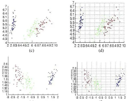
The IRIS data set was projected to three two dimensional subspaces. The first subspace used one vector from PCA and second vector from MDA corresponding to their highest Eigen values. The subspace is shown in Figure2a. The subspace was divided into 5 by 5 coarse grids as shown in Figure2b. The rules extracted from this coarse grid are shown below:

Rule 1: IF x-axis lies between 2.286 and 3.69 AND y-axis lies between 0.986 1.939

THEN class is 1 with probability of 1 Rule 2: IF x-axis lies between 3.690 5.094

AND y-axis lies between -0.921 0.032 THEN class is 2 with probability of 1 Rule 3: IF x-axis lies between 5.094 6.498

AND y-axis lies between -0.921 0.032 THEN class is 2 with probability of 1 Rule 4: IF x-axis lies between 6.498 7.902

AND y-axis lies between -2.828 -1.875 THEN class is 3 with probability of 1 Rule 5: IF x-axis lies between 7.902 9.306

AND y-axis lies between -1.875 -0.921 THEN class is 3 with probability of 1

Rule 7: IF x-axis lies between 5.094 6.498 AND y-axis lies between -1.875 -0.921

THEN class is 2 with probability of 0.947 Rule 8: IF x-axis lies between 6.498 7.902

AND y-axis lies between -1.875 -0.921

THEN class is 3 with probability of 0.629

The above coarse rules classify 132 examples out of 150 examples correctly giving a classification accuracy of 88%. The Rule 7 above corresponds to a grid that has examples belonging to two classes: class3 and class2. The proportion of examples belonging to class2 (i.e 18/19=0.947) and class3 (i.e. 1/19) is the probability with which this rule can classify a given example as belonging to class2 or class3 respectively. Similarly, the Rule 8 above corresponds to a grid that has examples belonging to two classes: class3 and class2. The proportion of examples belonging to class3 (i.e 17/27=0.629) and class2 (i.e. 10/27) is the probability with which this rule will classify a given example as belonging to class3 or class2 respectively.

Thus the grids corresponding to Rule 7 and Rule 8 have data belonging to more than one class and its use will result in classification error. To address this issue, the grids corresponding to Rule 7 and Rule 8 are divided into fine grids (each grid is divided into four grids). Rule 7 and Rule 8 are redefined by using fine grids. Note that it is not necessary that all new fine grids will have data in it, but those that do will give rise to redefined rules. The 8 new fine grids give rise to the following 4 rules:

Rule 7: IF x-axis lies between 5.796 6.498 AND y-axis lies between -1.398 -0.921 THEN class is 2 with probability of 1 Rule 8: IF x-axis lies between 6.498 7.20

THEN class is 3 with probability of 0.714 Rule 10: IF x-axis lies between 5.796 6.498

THEN class is 2 with probability of 0.5

The above set of rules classify 145 examples out of 150 examples correctly giving a classification accuracy of 96.7%. The Rule 9 above corresponds to a grid that has examples belonging to two classes: class3 and class2. The proportion of examples belonging to class3 (i.e 10/14=0.714) and class2 (i.e. 4/14) is the probability with which this rule will classify a given example as belonging to class3 or class2 respectively. Similarly, the Rule 10 above corresponds to a grid that has examples belonging to two classes: class3 and class2. The proportion of examples belonging to class3 (i.e 1/2 = 0.5) and class2 (i.e.1/2 = 0.5) is the probability with which this rule will classify a given example as belonging to class3 or class2 respectively.

(5)

(c) (d)

(e) (f)

Figure 2.(a,b) Subspace and grids using PCA and MDA algorithm (c, d) Subspace and grids using PCA algorithm, (e,f) Subspace and grids using MDA algorithm.

Thus the grids corresponding to Rule 9 and Rule 10 have data belonging to more than one class and its use will result in classification error. To improve the results further, Rule 9 and Rule 10 are refined by adding new premises. The new premises are obtained by using fine grids (10 by 10 grids) of other two projected subspaces: subspace 2 (using vectors from PCA algorithm) (Figure2c,d) and subspace 3 (using vectors from MDA algorithm) (Figure2e,f). Rule 9 gets modified as below:

Rule 9a: IF x-axis lies between 6.498 7.20 AND y-axis lies between -1.875 -1.398

THEN class is 3 with probability of 0.714 Rule 9b: (IF x-axis lies between 6.498 7.20

AND y-axis lies between -1.875 -1.398) from subspace 3 AND

(IF x-axis lies between -1.875 -1.398 AND y-axis lies between 1.394 1.540)

from subspace 2 THEN class is 2 with probability of 1 Rule 9c: (IF x-axis lies between 6.498 7.20

(IF x-axis lies between 6.498 7.20 AND y-axis lies between 5.368 5.632) from subspace 1 THEN class is 2 with probability of 0.83

Similarly, Rule 10 gets modified as below: Rule 10a: IF x-axis lies between 5.796 6.498

THEN class is 2 with probability of 0.5 Rule 10b: (IF x-axis lies between 5.796 6.498

(IF x-axis lies between -1.875 -1.398 AND y-axis lies between 1.540 1.687) from subspace 2 THEN class is 3 with probability of 0.75

The above set of rules classify 148 examples out of 150 examples correctly giving a classification accuracy of 98.67%. The classification accuracy results are summarized in Table 1 below:

TABLE I CLASSIFICATION ACCURACY WITH MULTI-SCALE SUBSPACE

GRIDS AND RULES ALGORITHM

Rules Used Classification

accuracy Rules from only Coarse Grids of subspace 3 88% Rules from Coarse and Fine Grids of subspace 3 96.7% Rules from Coarse and Fine Grids of subspace 3 with premises supplemented from subspaces 1 and 2.

98.67%

ii) Defect Recognition in Veneers of Wood

Seventeen different features are extracted from veneers of wood to represent tweleve different defects and clear veneer. Ten of these features are statistical features which give measure of central tendency, location, dispersion, symmetry and peaknedness of frequency distribution of grey level values under a window have been chosen for this task. Rest of the seven features are shape measures of the frequency distribution curve as explained below.

(i) Percentage of pixels in a window with grey level value of less than 80. This will differentiate the darker defects from the rest of the defects.

(ii) Percentage of pixels in a window with grey level value of more than 220. This will differentiate the brighter defects (under backlighting conditions) from the rest of the defects. (iii) Grey level value ‘a’ for which there are 2% pixels below it. This gives the dark end location of the frequency distribution curve.

(iv) Grey level value ‘d’ for which there are 2% pixels above it. This gives the bright end location of the frequency distribution curve.

(v) Histogram tail length on the dark side (b-a) where ‘a’ is defined in (iii) and ‘b’ is the grey level at which there are 20% pixels below it. This depicts the shape of the frequency distribution curve on its darker side.

(vi) Histogram tail length on the bright side (d-c) where ‘d’ is defined in (iv) and ‘c’ is the grey level at which there are 20% pixels above it. This depicts the shape of the frequency distribution curve on its brighter side.

(vii) Histogram length between the grey levels ‘b’ and ‘c’. This depicts the shape of the frequency distribution curve in the neighbourhood of its central point.

The seventeen dimensional feature vector was projected to a two dimensional space which was used as input to the neural network model for training. Table 2 gives summary the results of the wood defect recognition problem using the neural network models. A possible disadvantage with the synergistic neural network approach is that it needs training more than one neural network. However, if the structure of various neural networks of the proposed model is kept simple and identical then the task of training the neural networks becomes easier.

TABLE 2 CLASSIFICATION ACCURACY WITH MULTI-SCALE SUBSPACE

GRIDS AND NNALGORITHM

% Classification accuracy

Type of NN model

Simple 83.7

Synergistic 88.1

V. CONCLUSION

[image:5.595.58.281.52.228.2] [image:5.595.321.523.676.757.2]

(6)

data. Multidimensional data was projected to lower dimensional subspaces. The PCA and MDA algorithms were used to define lower dimensional subspaces. Coarse and fine grids were obtained from the lower dimensional subspaces by dividing the range of values associated with each vector of a subspace into equal number of parts. A rule based algorithm and a neural network based algorithm was used to recognize patterns using multi-scale subspace grids. The approach was tested on two applications. The paper showed that the use of multi-scale subspace grids to recognize patterns in multidimensional data produced good results.

REFERENCES

[1] H. Chai, H. and D. Domeniconi, “An Evaluation of Gene Selection Methods for Multi-class Microarray Data Classification”, Proceedings of the Second European Workshop on Data Mining and Text Mining in Bioinformatics. pp. 3-10, 2004.

[2] G. Hori, M. Inoue, S. Nishimura, and H. Nakahara, “Blind gene classification based on ICA of microarray data”, Proceedings of 3rd International Conference on Independent Component Analysis and Blind Signal Separation. San Diego. pp. 332-336, 2001.

[3] R. Pique-Regi1, A. Ortega, and S. Asgharzadeh, “Sequential Diagonal Linear Discriminant Analysis (SeqDLDA) for Microarray Classification and Gene Identification”, Proceedings of the 2005 IEEE Computational Systems Bioinformatics Conference–Workshop. pp. 112–116, 2005.

[4] H. Xiong, Y. Zhang, and X. Chen, “Data-dependent Kernel Machines for Microarray Data Classification”, IEEE/ACM Trans. Comput. Biology Bioinform. pp. 583-595, 2007.

[5] L. Wang, J. Zhu, and H. Zou, “Hybrid Huberized Support Vector Machines for Microarray Classification”, Proceedings

of the 24 th International Conference on Machine Learning. Corvallis, Oregon, pp 983-990, 2007.

[6] K. Kim, and S. Cho, “Ensemble classifiers based on correlation analysis for DNA microarray classification”, Neurocomputing, 70: pp. 187–199, 2006.

[7] S. M. Hosseyninia, F. Roosta, A. A. S. Baboli, G. R. Rad, “Improving the performance of MPCA+MDA for Face Recognition”, 29th Iranian Conference on Electrical Engineering, pp. 1-5, 2011.

[8] M. Arif Wani, “Incremental Hybrid Approach for Microarray Classification”, Proceedings of the Seventh International Conference on Machine Learning and Applications, San Diego, USA, pp. 514-520 , December, 2008.

[9] M. Arif Wani, "Microarray Classification using Subspace Grids", Proceedings of the Tenth International Conference on Machine Learning and Applications, Hawaii, USA, Volume 1, pp. 389-394 , December, 2011.

[10] R. A. Fisher, “The use of multiple measurements in taxonomic problems”, Ann. of Eugenics, 7, 179-188, 1936.

[11] M. Arif Wani, “Introducing Subspace Grids to Recognise Patterns in Multidimensinal Data”, International Conference on Machine Learning and Applications, Boca Raton, USA, IEEE publication, Volume 1, pp. 33-39, 2012.

[12] M. Arif Wani and D. T. Pham, “Efficient Control Chart Pattern Recognition Through Synergistic and Distributed Neural Networks”, Proceedings of Mechanical Engineers, Journal of Engineering Manufacture, pp 157-169, vol. 213, part B, 1999.