cells and their shapes. Specifically, we consider the deployment of an AP to provide terrestrial mobile radio communications using the universal mobile telecommunication system operating in its wide-band code-division multiple-access mode. Calculations are made of the number of users versus / 0 for different service rates. Multitiered cellular structures having cells of different size that are steerable with the offered teletraffic are examined. The array structure to achieve this is identified. The preliminary results shows that an AP at a height of 21 km covers an area of radius 517 km. Up to 21 users per cell with a service rate of 8 kb/s can be accommodated in the 2.2-GHz band. These services can be provided within an area of radius 70 km with transmitted powers of less than 1 W. High system capacity is proved to be possible by constructing cells of radius as small as 100 m using square planar arrays with dimensions of less than 12 m 12 m. The AP system provides high capacity and Doppler frequency shifts that only originate from roving mobiles.
Index Terms—Aerial platforms, cellular communications, code division multiple access (CDMA).
I. INTRODUCTION
W
ORLD-WIDE telephony and telegraphy supporting communications between fixed points has been avail-able for many decades. Today, people want at their disposal a wide range of multimedia services that they can use while on the move, or when stationary but not near a tethered terminal. Further, the number of people requiring mobile services is growing at an exponential rate. Consequently, networks in the twenty-first century will need to respond to rapid demands in offered traffic that are difficult to predict with regard to time and geography.The conventional way of designing a mobile network is to form cells of different shapes. This requires the acquisition of cell sites and the deployment of base-station (BS) equipment. Not only are BSs unable to respond to massive peaks in offered traffic, but they often spend a large fraction of the day in an idle state. For example, BSs in a business district may be very busy for ten hours a day, but when the business people depart, there is negligible offered traffic. The BS capacity cannot be switched elsewhere, such as to suburbia, where it is likely to be required. We therefore have a double problem. We do not know when or
Manuscript received September 4, 1998; revised July 19, 2000. This work was supported by the Secretariat of Education, Libya.
B. El-Jabu is with the Electrical Engineering Department, Al-Fateh Univer-sity, Libya, and the Higher Industrial Institute, Misurata, Libya.
R. Steele is with the Department of Electronics and Computer Science, Uni-versity of Southampton, Southampton SO17 1BJ, U.K.
Publisher Item Identifier S 0018-9545(01)03963-9.
To solve this problem, we need a different approach. In 1992, Steele proposed the use of stationary aerial platforms to handle moving peaks of teletraffic: “The platforms will be tethered to the earth and located up to 30 km in height and placed between the aircraft flying lanes. Barely visible from the earth they will be able to deliver many services. They will be held on station by power conveyed to them via their tie-lines, and these lines will also house the fibers that convey the teletraffic with the net-work. Alternatively these platforms could be untethered, hov-ering, and therefore capable of being rapidly re-deployed. The hovering platforms would communicate to earth via radio. The tethered or hovering platforms will be able to track ‘solitons of teletraffic,’ rather than force the task on to the terrestrial net-works. For example, the platforms could handle the teletraffic from high speed trains, highways, aircraft and ships. They can be rapidly deployed when disasters occur, for example, the rapid provision of communications to a city which has been devas-tated by an earthquake” [1]. Later, the application of aerial plat-forms for cellular networks was described in an editorial [2].
Since then, much has happened. Unmanned sky plat-forms have been proposed. The platplat-forms will consist of a multilayer skin airship having buoyant helium-filled cells, a station-keeping system, solar arrays for daytime power, and fuel cells for nighttime power. They will utilize a global positioning system for accurate position measurement, and ultrathin fabric hulls for long duration buoyancy [3].
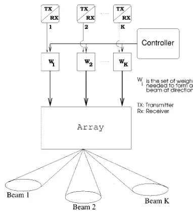
The deployment of aerial platforms (APs) using mul-tiple-beam phased array technology offers the prospect of deploying the network capacity when and where it is needed. Located at elevations of a few to 25 km or so, the APs are stationary and therefore do not contribute to Doppler frequency shift in radio transmissions. APs are sufficiently close to the earth that their path loss is low and compatible with those in conventional urban macrocells due to the free-space loss once the transmissions clear the city skyline. The capacity of APs can be high, as they are able to form small cells on the earth’s surface, as we will describe later, and have a good reuse factor. The APs can be moved to where they are required, when their elevation can be adjusted to suit network requirements. Moreover, they can be interconnected to form sky networks where APs are not only networked access nodes but also act as repeaters. Although an AP may form small cells by the use of multiple beams, they can also form megacells that span conventional terrestrial cellular structures [1].
This paper is concerned with the basic equations relating to aerial platform communications. Accordingly, we assume that
an AP is stationary, although we recognize that station-keeping is a far from trivial task. If an AP is an aircraft, such as the Pro-teus made by Angel Technologies, then it will fly in tight circles (some five to eight miles in diameter), with the station keeping about the center of the circle. We are not considering this type of AP in this paper. The airship type of AP must have suffi-cient propulsion to overcome stratospheric winds, which for a given location vary through the year. Even if sufficient propul-sion is available, there is still the problem of combatting the small vertical, lateral, and tilting movements. Positional insta-bility of APs has been studied [4], where it is shown that the tilt of an AP is the movement that has the most deleterious effect. If not restrained to less than 3 , it can significantly decrease the capacity of a code-division multiple-access (CDMA) AP net-work. However, as we are concerned here with basic equations and parameters, the stability issues will not be addressed.
II. THEVIEW OF THEEARTH FROM THEAERIALPLATFORM
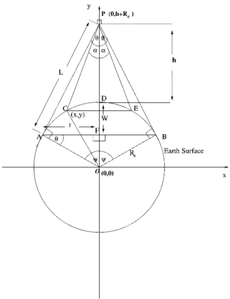
The extremities of the “view” of the earth’s surface from the aerial platform at point P in Fig. 1 is found by drawing a straight line from P to make a tangent with the earth’s surface at point A, and then rotating the arc AD by 360 about the -axis. The surface area mapped out is
(1)
where is the radius of the earth ( km) and is the depth from the earth’s surface, point D, that is immediately below P, to a plane within the earth surface that connects with points A and B. From triangle OAP, the distance from the plat-form to point A is
(2)
where is the nadir. From triangles FAP and OAF, we have
(3)
and
(4)
respectively, where is shown in Fig. 1. Eliminating from (3) and (4) and using (2) with obtained from (1) yields
(5)
For the situation where , i.e., square kilometers, . The variation of the radius of the total surface area covered by the aerial platform versus its height is displayed in Fig. 2.
The angle OPA in Fig. 1 is
(6)
and the curve from A to B is
[image:2.612.314.539.58.351.2](7)
Fig. 1. Cross-section atz = 0 in the space-earth geometry of the AP. The AP is at position P.
The straight line AB, which passes through point F, is given by
AB (8)
To approximate the curve AB through D by the straight line AB, the following condition should be satisfied:
(9)
Using the fact that for , (9) is valid if , when
(10)
or km.
Consider point C on the earth’s surface, having the coordi-nates referenced to the center of the earth, as shown in Fig. 1. The distance from the platform to point is
PC (11)
for and . Substituting from the
previous equations for and , the length PC becomes
PC (12)
and the arc CD is
Fig. 2. The height of the AP versus the radius of the maximum area covered on the earth’s surface.
Fig. 3. Communications via multibeams in the AP system.
The total angle coverage of the platform ( ) is 2 and can be evaluated from
(14)
The angle in Fig. 1 is
(15)
while the surface area containing CDE is
(16)
and
(17)
III. MULTIBEAMANTENNA
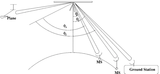
The aerial platform will support a multibeam antenna. One beam will be directed at all times to the fixed network ground station that is connected to the cellular network. The other beams will be directed to fixed ground sites if they provide back-haul links from ground macrocellular or microcellular systems; or they will be steerable beams if they have to accom-modate mobile traffic, which varies in location and intensity hour by hour. These steerable beams provide the network’s capacity-on-demand feature. Fig. 3 shows a number of beams, including one that is tracking an airplane and offering the pilot and passengers communication links to a global network, e.g., to the Universal Mobile Telecommunication Services (UMTS) global network.
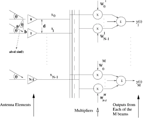
[image:3.612.130.468.344.500.2]Fig. 4. Beamforming at the AP receiver.
between each two adjacent elements, which generates re-ceiving beams.
Let us consider the reception of signals from the ground. Be-cause the source is in the far field, the received rays are parallel. The differential distance along the two ray paths is , where is an arbitrary angle of arrival ( ). Notice that the angle of arrival is different for each beam, and Fig. 4 displays the arrival of only one beam. Each element is weighted with a complex weight , with
and . Assuming that the phase of the received ray at antenna element 0 is zero, the output of beam of the array is
(18)
where
(19)
and is the speed of light. Substituting from (19) into (18) yields
(20)
where , is the wavelength, and
(21)
is the array factor.
Let the phase of the th element lead that of the ( 1)th element by . On introducing a weight factor for the
th beam, element , we have
(22)
Accordingly, the th array factor becomes
(23)
The beam shape depends on the weights. Assuming a uniform distribution, i.e., all of the weights have the same magnitude,
for all . Using the formula gives the array factor
(24)
the absolute value of which is
(25)
For the th beam to be at an angle , , and the power pattern of this array in the direction becomes
(26)
which has a maximum gain of .
By controlling the magnitude of the weights and the number of elements, the gain of each beam can be controlled, with each beam having ( 2) side lobes. The phase of the weights are used to control the direction of the main beam. The nulls of the main beam are obtained from (26) when
(27)
from which the width of the main beam between zeros is
(28)
Thus, the beamwidth depends on the number of elements, the distance between them (relative to the wavelength), and the di-rection of the beam. In this context, the following points are worth mentioning.
1) Equation (26) repeats every 2 radians, and so more than one main beam in the visible region may occur. To avoid this, the spacing should always be kept less than . 2) For a given number of elements, increasing the spacing
between them decreases the beamwidth and increases the array size ( ).
Fig. 5. Three beams at030 , 0 , and 60 formed by a ten-element linear array.
Fig. 6. Beamforming at the AP transmitter.
have different beamwidths. The patterns are symmetrical about the axis of the array.
Generally, the 3-dB beamwidth is obtained by solving (26) numerically, although there are some approximated formulas for special cases [5].
Let us now consider generating the multibeams for transmis-sion. The weights now control the magnitude and the phase dif-ference of the currents fed to the elements, as indicated in Fig. 6. If the weights are chosen such that , then the power pattern of the beam directed at an angle becomes
(29)
which has a maximum gain of .
Fig. 7. Two-dimensional array ofN 2 M elements.
A. Two-Dimensional Arrays
A rectangular or planar array consists of and elements along the and ordinates, respectively, as shown in Fig. 7 [5]. This array may be viewed as linear arrays, and the two-dimensional (2-D) array factor is found by multiplying the array factor for the arrays along the axis by the array factor for the dipoles along the axis [6], i.e.,
(30)
(31)
and
(32)
where is the overall array factor with
and . In (30) and (31),
is the phase shift between the elements in the -axis, while is the phase shift between the elements in the -axis.
Repeating the steps of the one-dimensional case, and for a uniform array, the array factor of the 2-D array directed toward ( , ) is
(33)
For a large array, where the beams are close to the broadside, the elevation plane half-power beamwidth (HPBW) is given ap-proximately by [5]
BW
[image:5.612.42.289.347.512.2]Fig. 8. Three-dimensional pattern for square array of 102 10 elements with spacingd = =2 directed toward (0,0).
where and represent the half-power bandwidths. For a
square array ; , ; and
s s (35)
For the plane that is perpendicular to the elevation, the half-power beamwidth is
BW (36)
which reduces to
BW (37)
for a square array.
As an example, consider a square array of 10 10 elements where the distance between each two elements on the same row or the same column is . This array produces a three-dimensional pattern directed toward (0,0), as shown in Fig. 8. However, this pattern may be modified to electronically steer the central beam as required. An identical pattern is formed in the lower hemisphere, which can be diminished by the use of a ground plane [5].
IV. FORMULATION OFCELLS
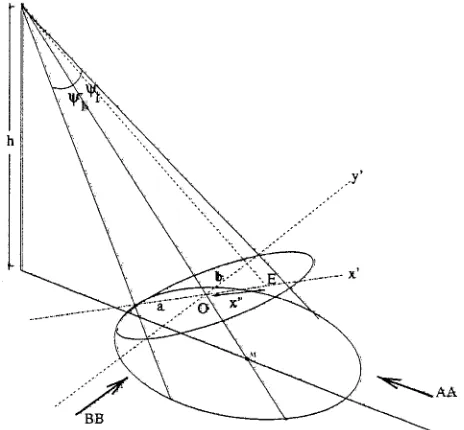
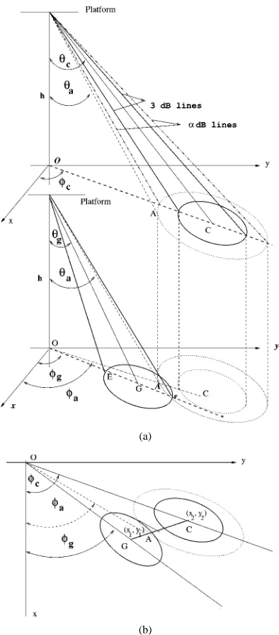
We now examine how we form cells on the earth’s surface using an AP. Consider first the formulation of a single cell by a beam from a multibeam antenna system connected to the un-derside of the AP. The beam at an angle ( , 0) from the AP delivers a footprint on the earth’s surface, as shown in Fig. 9. This footprint corresponds to the half-power beamwidth, and we refer to this footprint as a single cell. Beyond this footprint, the coverage decreases with distance and constitutes interference in neighboring cells formed by other beams.
Referring to Fig. 9, the equation of the footprint for a beam with elevation plane half-power beamwidth BW and
Fig. 9. The geometry of a footprint of a beam on the earth’s surface from an AP.
half-power beamwidth BW , in the plane that is perpen-dicular to the elevation, is shown in Appendix 1 to be
(38)
where . If a point
is rotated by an angle , the new coordinates, which are due to a beam directed toward ( , ), becomes
(39)
and
(40)
When and , the equation is that of a circle of radius , where is half of the half-power beamwidth of the broadside beam.
Let us consider an AP with a square array of 10 10 elements with . As data from worldwide measurements of strato-spheric wind velocities indicate that their minimum averages from 30 to 40 m/s occur between 65 000 and 75 000 ft (19–23 km) depending on the latitude [7], we will consider the platform to be at a height of 21 km throughout this paper. The broadside half of the half-power beamwidth of this array is found numer-ically to be 5.1 , and the corresponding broadside cell radius is 1.876 km. To find the footprints of different beams in different directions, we take into account the change of the beamwidth as the scanning angle changes by introducing a continuous func-tion. To arrive at this continuous function, we first determined
numerically the HPBW at , , , , , and
[image:6.612.53.277.64.237.2]Fig. 10. The HPBW versus scanning angle for the exact results, using the approximation formula and the curve fitting procedure for a square array of 102 10 elements with spacingd = =2.
Fig. 11. Cell structure on the earth’s surface for a square array having 102 10 elements with spacing d = =2 (dimensions of both axes in km).
curve fitting was applied to the exact curve at the values to yield the continuous function of the half of the HPBW
(41)
where (but converted to radians), such that is the direction of the main beam in the -direction. This function
[image:7.612.113.485.353.655.2](a)
[image:8.612.65.262.58.505.2](b)
Fig. 12. Geometries employed in cochannel interference calculations.
V. CONTIGUOUSCELLS
An AP at a height of km transmits and receives contiguous spot beams that form cells on the earth’s surface. Each cell is defined here as an area within the HPBW coverage. Consider a mobile station (MS) located at point A in Fig. 12, which is km from the platform with direction ( , ) measured from the position of the platform. This point is covered by a beam directed toward point G at direction ( , ).
Let the power transmitted by the AP in each beam (i.e.,to each cell) be . On assuming free-space propagation, the power re-ceived by a terminal at point A is
(42)
where is the gain of the receiving antenna of the terminal and is the gain of the beam covering the cell con-taining point A evaluated in the direction ( ). As the HPBW
defines the cells, some energy is radiated into neighboring cells. The interference received by the MS from the main beam cov-ering the cell centered at C is given by
(43)
where the subscript signifies interference and
is the gain of the beam directed toward point C evaluated at . The signal-to-interference ratio (SIR) at the MS is found from (42) and (43) as
SIR (44)
For interfering cells, the total SIR is given by
SIR (45)
where is the beam gain of the th interfering cell evaluated at . For each service, the SIR should exceed a minimum value SIR . To fulfill this obligation, the following inequality should be satisfied:
SIR (46)
The SIR of (45) can be calculated along a line connecting the centers of any two cochannel cells. Then the cell structure that satisfies the conditions in (46) can be determined. Assuming that the coordinate of point G in Fig. 12 is ( ), and that of point C is ( ), then the equation of line GC is
(47)
where such that
(48)
from which the other distances and angles can be found as
GA (49)
(50)
OA (51)
(52)
The SIR and the required cell structure will be calculated for an AP at a height of 21 km employing a square array of 10 10 elements such that the distance between each two elements is
.
1) Single Cell Per Cluster: Assume that the AP is used for
Arranging for all the beams to have the same maximum gain, i.e., for all and
(53)
and
(54)
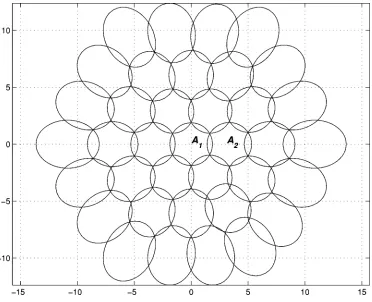
which is the gain of the beam of the interfering cell directed to-ward C evaluated at . By selecting A, the maximum gain of the main beam is 30 dB as the array dimen-sions are 10 by 10. Arranging for one cell per cluster, the gain of the main beam in Fig. 11 as a function of the distance from the center of along a line to the center of (also in Fig. 11) is shown by the solid line in Fig. 13(a). We emphasise that the the same frequencies are used in cells and . Also displayed in Fig. 13(a) is the curve representing the variation of the gain of the main beam for . Defining a cell as the 3-dB beamwidth, we note that the boundary of is at about 1.9 km (similar to the previous calculations), while the boundary of commences at about 1.4 km.
(a)
[image:9.612.70.261.84.274.2] [image:9.612.40.288.316.600.2](b)
Fig. 13. Results for one cell per cluster.
Fig. 13(b) shows the variation of SIR experienced by an MS assigned to as it travels the same distance in Fig. 13(a). The interference is computed not just from cell but from all the cells that form a ring around , assuming one user per cell. Observe that at the cell boundary of , the SIR is about 3.5 dB, and hence this cell cluster arrangement is only suitable for CDMA, and not time- or frequency-division multiple access.
In digital systems, the SIR at the receiver input is closely re-lated to at baseband, namely [9]
SIR (55)
where
energy per bit;
interference power spectral density (PSD) in watts/ Hertz;
message data rate in bits per second;
user contributes the same amount of interference such that the total SIR becomes
SIR
(56)
or
SIR (57)
where
(58)
is the inverse of the total SIR experienced by the mobile in the cell under considerations from the cochannel cells, assuming one mobile per cochannel cell [it is the inverse of (45)]. The value of can be obtained with the help of Fig. 13(b).
Equating (55) and (57) and solving for gives
(59)
where we observe that the number of users decreases as in-creases. The worst case is on the cell boundary, when rep-resents the lower bound of the number of users the system can accommodate, assuming the other variables of (5) are constants. Consider the central cell, from Fig. 13(b), dB on the boundary of the central cell. Using this value for and for MHz, (59) was calculated as a function of for different service rates. The results are displayed in Fig. 14(a). The same equation was calculated as a function of the service rate for different values of / , and the results are displayed in Fig. 14(b). From Fig. 14(a), we observe that the system can ac-commodate more than 160 users having a service rate of 8 kb/s if the required is 0.2 dB, and 30 users if dB. These numbers drops to 40 and eight users, respectively, if the service rate is increased to 32 kb/s. From Fig. 14(b), the number of users decreases sharply as the service rate increases above 32 kb/s.
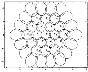
2) Three Cells Per Cluster: When the procedure is applied
for the three cells per cluster arrangement shown in Fig. 15, we obtain the variation of the gain of the main beam , and the main beam toward , as a function of distance measured along the line connecting the two cells. The result is shown in Fig. 16(a). From Fig. 15, we calculate the interference experi-enced by the central cell from cells , , , , , and . The SIR is found next, and its variation with distance is shown in Fig. 16(b). From Fig. 16(a), the boundary of the central cell is also at approximately 1.9 km, while the boundary of the cell is at about 4 km. From Fig. 16(b), the corresponding distance to SIR dB is 2 km. As this distance is between
(a)
[image:10.612.310.541.60.454.2] [image:10.612.39.287.88.278.2](b)
Fig. 14. Minimum number of users with UMTS CDMA.
Fig. 15. Cell structure for square array of 102 10 elements with spacing d =
=2 with a reuse factor of three. Dimensions are in kilometers.
the boundaries of and , we conclude that three cells per cluster are also suitable for third-generation TDMA systems.
VI. CELLS WITHVARIABLESIZES ANDLOCATIONS
[image:10.612.332.519.486.638.2](a)
[image:11.612.304.554.60.485.2](b)
[image:11.612.52.280.64.458.2]Fig. 16. Results for three cells per cluster.
Fig. 17. Arrangements to change cell size and location.
in Fig. 17. The controller changes the phase of the weights ac-cording to the required direction, the number of weights to the
(a)
(b)
Fig. 18. Cell forming according to traffic.
size(number of connected elements of the array) according of the cell, and the values of the weight to adjust the gain of the beam.
[image:11.612.66.257.490.699.2]Fig. 19. The required transmitted power versus the radius of the area covered for different chip rates.
VII. TRANSMISSIONRATE ANDDELAY
The maximum propagation time delay of a signal trans-mitted by the platform can be calculated as
(60)
where is the speed of light ( m/s) and is the distance shown in Fig. 1 and given by (2).
Delay is an important factor in global communications. It is interesting to compare the delay of an AP network with the delay incurred in a fiber link. To make this comparison, we consider the arc length AB in Fig. 1, as it is the maximum distance be-tween two mobiles. The distance using optical transmission is the length of the arc AB. Applying (7) for ,
, yielding the arc for
km. For the AP, the maximum distance travelled by a signal is 2 517 km for a platform at 21 km. The optical signal travels almost the same distance. However, the propagation of light in fiber depends on its dielectric constant. If it is 2 10 m/s com-pared to 3 10 m/s for the velocity of light, the time taken to travel arc AB for the optical fiber link and for the AP links is 5.2 and 3.5 ms, respectively.
When transactions are relatively local, then delay constraints can be relaxed, but attention must be given to the minimization of delay when we are considering transactions on a global basis. As an example, for an ocean of 6000 km, a geostationary link is 250 ms, a fiber of length 10 000 km (to allow for variations on the ocean floor) is 50 ms, while if we establish a network of sky platforms [3] at 20 km above the ocean, spaced 1 km apart, the delay is only 23 ms, ignoring the relaying process delay in each sky platform [10]. Low-earth-orbit satellites have delays only a little greater than those of sky platform transmissions, but they have disadvantages of a relatively low capacity and high Doppler frequency shifts [10].
For a digital free-space channel, the bit energy per noise power spectral density is given by [11]
(61)
where
transmission rate in bits per second; receiver temperature in degrees Kelvin; Boltzmann’s constant ( J/K); free-space loss;
summation of other losses (e.g circuits losses); link margin.
The free-space loss is expressed as [11]
(62)
where is the link distance and is the wavelength. Expressed in decibels, (61) becomes
dB dB dB dB
and the free-space loss (62) becomes
(63)
where is the operating frequency in hertz and is the link distance in meters. The link distance depends on the location of the station measured from the AP and is calculated using (11).
Fig. 20. Array size as a function the radius of the central cell at 21 km and 2.2 GHz.
an isotropic antenna for mobile station. The transmitted power as a function of the radius of the total area covered is displayed in Fig. 19. Observe that an AP at a height of 21 km can cover an area of radius 70 km with a chip rate of up to 16.384 Mc/s using 0 dB (1 mW) transmission power.
VIII. ARRAYSTRUCTURESIZE
As an adaptive antenna array system will be used on the AP, the structure size is of importance. For large square arrays, the broadside 3-dB beamwidth (HPBW) is approximated by [6]
(64)
The radius of the broadside cell (the central cell) formed by an AP at height is
(65)
where BW and is the size of the array. Substituting for , the size of the array may be calculated using
(66)
For a specified , increasing the height of the AP requires a larger array. However, the array size decreases as the operating frequency increases. The array size as a function of the radius of the central cell for km, assuming operating frequency of 2.2 GHz, is shown in Fig. 20. From this figure, it is clear that the size of the arrays needed in the AP system is realizable.
IX. CONCLUSION
With the expected deployment of third-generation (3G) net-works starting in 2002, the application of aerial platforms in 3G is very attractive. For our part, we have conducted a pre-liminary analysis that gives us optimism that aerial platforms have a future role to play in supporting 3G terrestrial multi-media networks. They have the ability to provide multiple cells via the adaptive multibeam antenna arrays they have on-board; to change the beam size to form cells as small as 100 m, i.e., form microcells; and to generate large cells of many kilometers if required. The platforms are stationary so they do not introduce any changes in Doppler frequency, they are at a sufficiently low altitude that propagation delays are only a few milliseconds, and their capacity can be very high because they can operate CDMA links with a reuse of unity. The movement of the beams means the cells move, and if necessary, simultaneously change in size. Therefore, the infrastructure can be electronically reorganized to suit the changing teletraffic patterns of mobile users. Notice that the cost of terrestrial base stations and site rentals is now transformed to the cost of the aerial platforms.
(a) (b)
[image:14.612.56.545.53.790.2](c)
Fig. 21. Geometry for one beam from the AP.
APPENDIX A
FOOT-PRINT OF THEAP BEAMS
From Fig. 21(c), the distance is given by
(A.1)
and
OC (A.2)
where . Also
(A.3)
The equation of the ellipse formed by intersection of the beam with the plane is
(A.4)
where
OC (A.5)
and
OC (A.6)
from which
(A.7)
From the projection in Fig. 21(c)
(A.8)
The line OC CM-MO, so
(A.9)
Substituting (A.5) into (A.9) and solving for OC leads to
OC (A.10)
From Fig. 21(b)
(A.11)
and
DC EF
Substituting the formula
(A.15)
into (A.14), and upon using
sec (A.16)
we have
(A.17)
To measure taking point as a reference, the distance should be added to (A.1) so the new becomes
(A.18)
Substituting this last equation into (A.17) gives the locus of the beam on the ground as
(A.19)
where . If a point
is rotated by an angle , the new coordinates will be
(A.20)
and
(A.21)
ACKNOWLEDGMENT
The authors acknowledge the discussions with Dr. D. Nunn, D. Stewart, and S. L. Dhomeja from the Department of Elec-tronics and Computer Science, University of Southampton, U.K. They are also grateful to B. Sultan, Department of
platform on its CDMA performance,” in Proc. VTC’99 Fall, Amsterdam, The Netherlands, Sept. 1999.
[5] C. A. Balanis, Antenna Theory: Analysis and Design. New York: Harper Row, 1982.
[6] R. E. Collin, Antenna and Radio-wave Propagation. New York: Mc-Graw-Hill, 1985.
[7] G. M. Djuknic, J. Freidenfelds, and Y. Okunev, “Establishing wireless communications services via high-altitude aeronautical platforms: A concept whose time has come,” IEEE Commun. Mag., pp. 128–135, Sept. 1997.
[8] ETSI/SMG/SMG, The ETSU UMTS Terrestrial Radio Access (UTRA) ITU-R RTT candidate submission, , 1998.
[9] W. C. Y. Lee, “Overview of cellular CDMA,” IEEE Trans. Veh.Technol., vol. 40, pp. 291–302, May 1991.
[10] R. Steele, “Communications++: Do we know what we are creating?,” in
Proc. EPMCC’97, VDE-VERLAG GMBH, Berlin, Germany, Sept. 1997,
pp. 19–23.
[11] B. Sklar, Digital Communications: Fundamentals and
Applica-tions. Englewood Cliffs, NJ: Prentice-Hall, 1988.
Bashir El-Jabu was born in Misurata, Libya, in 1957. He received the B.Sc.
degree in electrical engineering from Al-Fateh University, Libya, in 1980, the M.Sc. degree in electrical engineering from Queens University, Canada, in 1986, and the Ph.D. degree in electronics from the University of Southampton, Southampton, U.K., in 1999.
He is an Assistant Professor in the Electrical Engineering Department, Al-Fateh University, Libya, and Head of Scientific Department at the Higher Industrial Institute, Misurata, Libya. His current research interests are mobile communications and signal processing. He has published many papers in the field of communications, signal processing, and education.
Raymond Steele (SM’80–F’96) is Chairman of Multiple Access
Communica-tions Ltd., a company he formed in 1986 that is concerned with consultancy and products in digital mobile radio systems. His former posts were as Head of the Communications Research Group in the Department of Electronics and Computer Science, University of Southampton; a Research Worker with Bell Laboratories; a Research and Development Engineer with the Marconi Com-pany, Cossor Radar & Electronics, and E. K. Cole Ltd.; and a Senior Lecturer at the University of Loughborough. He is the author of Delta Modulation
Sys-tems (New York: Halsted, 1975), editor of Mobile Radio Communications (New
York: IEEE Press and Wiley, 1992), coauthor of Source-Matched Mobile
Com-munications (New York: IEEE Press and Wiley, 1995), and author of more than
200 technical publications. He has been a Conference and Session Organizer of numerous international conferences and a Keynote Speaker at many inter-national meetings. He is a member of the Advisory Board of the Interinter-national
Journal of Wireless Information Networks.
Prof. Steele is a Fellow of The Royal Academy of Engineering and the IEE, U.K. He is a Member of the IEEE Avant Garde and is an IEEE Distinguished Speaker. He is a Member of the Advisory Board of IEEE Personal
Communi-cations (the magazine of nomadic communiCommuni-cations and computing). He and his
coauthors received the Marconi Premium in 1979 and 1989 and the Bell System
Technical Journal’s award for the Best Mathematics, Communications,