detector (MUD) is considered for direct sequence code division multiple access (DS-CDMA) signals transmitted through multi-path channels. The emerging learning technique, called support vector machines (SVMs), is proposed as a method of obtaining a nonlinear MUD from a relatively small training data block. Com-puter simulation is used to study this SVM MUD, and the results show that it can closely match the performance of the optimal Bayesian one-shot detector. Comparisons with an adaptive radial basis function (RBF) MUD trained by an unsupervised clustering algorithm are discussed.
Index Terms—Direct sequence code division multiple access
(DS-CDMA), linear MMSE detector, multiuser detector (MUD), mul-tiuser interference, optimal one-shot detector, support vector ma-chines, unsupervised clustering.
I. INTRODUCTION
D
IRECT-sequence code-division multiple-access (DS-CDMA) [1] constitutes an attractive multiuser scheme that allows users to transmit at the same carrier fre-quency in an uncoordinated manner. However, this creates multiuser interference (MUI) which, if not controlled, can seriously degrade the quality of reception. Mutually orthogonal spreading codes for different users can provide an inherent immunity to MUI in the case of synchronous systems. Un-fortunately, multipath distortions are often encountered in DS-CDMA systems and will reduce this inherent immunity to MUI. A variety of receivers, known as multiuser detector (MUDs), have been proposed for DS-CDMA systems [2]–[4]. In a DS-CDMA system, the objective of the receiver is to detect the transmitted information bits of one (at mobile-end) or many (at base station) users. In this paper, the first case is considered. This is usually referred to as the downlink scenario, the com-munication channel from base station to mobile. In particular, the one-shot detector, that is, the receiver detecting a user bit at a bit period, is studied. Furthermore, we will concentrate on the scenario where a few strong interfering users exist, as the use of an MUD is especially effective in such a situation.For such applications, the linear minimum mean square error (MMSE) MUD [5]–[9] is widely used, as it is computationally very simple and can readily be implemented using standard adaptive filter techniques. A more complicated linear minimum bit error rate MUD has also been studied [10]–[14]. Linear de-tectors, however, can only work when the underlying noise-free signal classes are linearly separable. As nonlinear separable
Manuscript received April 7, 2000; revised October 23, 2000.
The authors are with the Department of Electronics and Computer Science, University of Southampton, Highfield, Southampton SO17 1BJ, U.K. (e-mail: [email protected]).
Publisher Item Identifier S 1045-9227(01)04161-3.
have been considered as nonlinear MUDs. In the work [15], a multilayer perceptron (MLP) was applied to a CDMA system without intersymbol interference (ISI). The experience shows that the MLP MUD has better performance than the linear MUD but training times are long and unpredictable. Mitra and Poor [16] applied a RBF network to the same problem. An advantage of the RBF MUD is its intimate link with the optimal one-shot detector. Training times are better and more predictable than the MLP. A RBF receiver [17] was also considered for channels with memory, and a Volterra series detector was explored [18].
A learning technique known as the SVM has recently gaining popularity due to its many attractive features and promising empirical performance [19]–[26]. The formulation of SVM embodies the structural risk minimization (SRM) principle, as opposed to the empirical risk minimization (ERM) approach commonly employed in statistical learning. SRM minimizes an upper bound on the generalization error, as opposed to ERM which minimizes the error on the training data. It is this differ-ence which equips SVMs with a greater potential to generalize. For binary classification tasks, the SVM approach nonlinearly maps the input space into a high-dimensional feature space via simple kernel representations. In the high-dimensional feature space, a linear classifier with maximum margin is constructed. Apart from good generalization properties, the learning aspect of SVMs is intriguing. An SVM classifier is determined only by a sparse set of support vectors (SVs), and these SVs are automatically selected from the training data during the learning process.
The SVM technique has been applied to channel equalization [27]–[30]. These studies have shown that the SVM approach is very effective in overcoming ISI and cochannel interference. As the idea of SVM is originated from finding an optimum hy-perplane to separate two classes with maximum margin, it is also very relevant to multiuser detection in DS-CDMA. In this paper, the SVM technique is investigated as an adaptive non-linear MUD. Our study shows that an SVM MUD trained using a relatively small block of noisy received signal samples can closely approximate the optimal MUD which requires a com-plete knowledge of the system. The remainder of the paper is organized as follows. Section II presents the DS-CDMA system model used and provides the necessary notations and defini-tions. Section III summarizes the linear MMSE MUD and the optimal Bayesian one-shot MUD. In Section IV, the proposed SVM MUD is presented. Section V gives some computer sim-ulation results, comparing the performance of the SVM MUD with those of the linear and optimal MUDs. Section VI com-pares the adaptive SVM MUD with a RBF MUD trained by
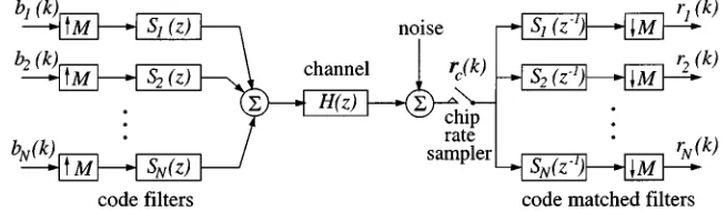
Fig. 1. Discrete-time model of synchronous CDMA downlink.
an unsupervised clustering algorithm [31]–[34]. The paper con-cludes in Section VII.
II. SYSTEMMODEL
Using notations from the multirate filtering literature [35], the discrete-time model of the synchronous DS-CDMA system with users and chips per bit is depicted in Fig. 1, where denotes the th bit of user , the signature code sequence for user
(1)
is normalized to have a unit length, and the transfer function of the channel impulse response (CIR) is
(2)
It is assumed that . The bit vector of users at is
(3)
and the received signal vector after the chip-matched filters is
(4)
The baseband model for can be represented by [36]
. .. ... ..
. . .. . ..
.. .
.. .
(5)
where the channel white Gaussian noise vector is
with
(6) the user signature sequence matrix is
(7)
the diagonal user signal amplitude matrix is
(8)
that is, is the user signal power; the CIR matrix has the form
. .. . .. . .. (9)
the system matrix is defined by
. .. ... ..
. . .. . ..
(10)
and orthogonal code sequences are assumed, so that the noise vector at the outputs of the chip-matched filters is
with
(11) The ISI span depends on the length of the CIR, , related to the length of the chip sequence, . For , ; for
, ; for , ; and so on.
The model (5) adopted in this study can readily be extended to the more general case of asynchronous DS-CDMA systems by an appropriate expansion of the system matrix [6].
where
(14)
denotes the detector weight vector for user . The most popular solution for the detector (13) is the MMSE solution given by
(15)
where is the th column of . The linear detector (13) is computationally very simple, and standard least mean square (LMS) or recursive least squares (RLS) algorithms can be used to implement the MMSE solution adaptively.
However, a linear MUD only performs adequately in certain situations. Let the possible combinations or
se-quences of be
.. .
(16)
and the th element of . Define the set of the noise-free received signal states as
(17)
can be partitioned into two subsets
(18)
If and are not linearly separable, a linear MUD will have an irreducible error floor even in the noise-free case, as it can only form a hyperplane in the -dimensional received signal space.
As the one-shot MUD at a bit period is only concerned with one particular bit from one particular user, the optimal solution can be derived from a one-shot Bayesian classification problem, similar to the channel equalization problem [31]. Thus, the op-timal one-shot detector for user can readily be given as
(19) where are a priori probabilities of and serve as class labels. Usually, all the are equiprobable, and
. The optimal decision is then given by
(20)
IV. THESUPPORTVECTORMACHINEDETECTOR
The optimal detector (21) requires the knowledge of all the noise-free signal sates , which are unknown to receiver . In general, the receiver can have access to a block of training
samples . For notational convenience, let
and , and denote the training set of noisy received signal vectors as
(22)
and the set of corresponding class labels as
(23)
Applying the standard SVM method [19], an SVM detector can be constructed for user
(24)
where the set of Lagrangian multipliers , denoted in the vector form
(25)
is the solution of the quadratic programming (QP)
(26) with the constraints
(27)
and
(28)
In this particular application, it is obviously advantageous to choose the Gaussian kernel function
(29)
received signal space and possesses certain symmetric proper-ties due to the symmetric structure of and , can be used. With this choice of the offset constant, the equality constraint (28) is no longer needed, and this leads to a simpler optimization task. The user-defined parameter controls the tradeoff between model complexity and training error. In our application, we will choose empirically.
The set of SVs, denoted by , is given by those s with nonzero Lagrangian multipliers . is usually a small subset of the training data set . These SVs are deter-mined during the optimization process. Thus the SVM MUD consists of computing the decision variable
(30)
and making the decision with
(31)
Before presenting some simulation results, we emphasize that the main purpose of this study is to investigate feasibility of the SVM method as a nonlinear MUD, and we use the standard gra-dient method to solve for the QP problem (26). Such an opti-mization technique associated with the SVM method requires a considerable amount of computation, especially for a large . The issue of computational efficiency is more general than the MUD problem. Efficient SVM implementation is an active area of research (see, for example, [23], [37], and [38]).
V. SIMULATIONRESULTS
Two simulation examples were used to investigate the pro-posed SVM MUD and compare its performance with those of the linear MMSE and optimal MUDs. It is worth pointing out again that the linear MMSE MUD and the optimal MUD are designed based on the complete knowledge of the system (the system matrix and the noise variance) while the SVM MUD is trained using a block of the noisy received signal samples.
Example 1: This was a two-user system with four
chips per bit. The code sequences of the two users were
and , respectively, and
the transfer function of the CIR was
(32)
The two users had equal signal power, that is, the user 1 signal to noise ratio (SNR ) was equal to that of user 2 (SNR ). Fig. 2 depicts the two subsets of noise-free signal states for user 1 to-gether with the decision boundaries of the linear MMSE and optimal Bayesian MUDs, given SNR SNR dB. It is clear that for user 1 it is not worth to implement a complex nonlinear detector, as a simple linear detector can perform ade-quately. However, for user 2, and are not linearly sep-arable and the linear MMSE detector will have an irreducible error floor of 0.125, as illustrated in Fig. 3.
[image:4.612.339.516.62.218.2]Fig. 2. The set of noise-free signal points and the two decision boundaries (dotted: linear MMSE, solid: optimal) for user 1 of Example 1. SNR = SNR = 16 dB.
Fig. 3. The set of noise-free signal points and the three decision boundaries (dotted: linear MMSE, thick solid: optimal, thin solid: SVM) for user 2 of Example 1. SNR = SNR = 20 dB.
TABLE I
INFLUENCE OFCONCONSTRUCTING THESVM MUDFORUSER2OF
EXAMPLE1. SNR = SNR = 20 dB,AND THENUMBER OF
TRAININGDATAIS160
TABLE II
INFLUENCE OFCONCONSTRUCTING THESVM MUDFORUSER2OF
EXAMPLE1. SNR = SNR = 15 dB,AND THENUMBER OF
TRAININGDATAIS160
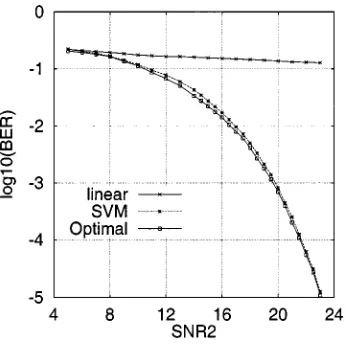
[image:4.612.345.510.274.419.2]Fig. 4. Performance comparison of three MUDs for user 2 of Example 1. SNR = SNR , and the training data set for SVM has 160 samples.
Fig. 5. Performance comparison of two MUDs for user 1 of Example 2. SNR ,
1 i 3, are identical.
the construction of SVM model, but the solution is not overly sensitive to it. The decision boundary of the constructed SVM MUD for user 2 is compared with those of the linear MMSE and optimal MUD in Fig. 3, given SNR SNR dB. Fig. 4 plots the BERs of the three MUDs for user 2 under different noise conditions. The results clearly show that the SVM MUD can closely match the performance of the optimal one-shot de-tector. For the given training set of 160 points, the number of SVs were found typically to be around 40.
Example 2: This was a three-user system with eight
chips per bit. The code sequences for the three users were
, , , , ,
and , , ,
respectively, and the transfer function of the CIR was
(33)
[image:5.612.339.512.278.449.2]The three users had equal signal power. For user 1, the perfor-mance of the linear MMSE detector is very close to the optimal detector, as shown in Fig. 5. For users 2 and 3, however, non-linear MUDs are certainly needed, as can be seen in Fig. 6 and Fig. 7.
[image:5.612.78.248.279.447.2]Fig. 6. Performance comparison of three MUDs for user 2 of Example 2. SNR ,1 i 3, are identical, and the training data set for SVM has 640 samples.
Fig. 7. Performance comparison of three MUDs for user 3 of Example 2. SNR ,1 i 3, are identical, and the training data set for SVM has 640 samples.
TABLE III
INFLUENCE OFCONCONSTRUCTING THESVM MUDFORUSER2OF
EXAMPLE2. SNR = 30 dBFOR1 i 3,AND THENUMBER OF
[image:5.612.306.543.515.684.2]TRAININGDATAIS640
TABLE IV
INFLUENCE OFCONCONSTRUCTING THESVM MUDFORUSER2OF
EXAMPLE2. SNR = 25 dBFOR1 i 3,AND THENUMBER OF
TRAININGDATAIS640
training data set of 640 points, typically around 200 SVs were selected. The BERs of the resulting SVM MUDs for users 2 and 3 are given in Figs. 6 and 7, respectively, in comparison with the corresponding linear MMSE and optimal one-shot MUDs. The results again demonstrate that the SVM MUD can closely approximate the performance of the optimal detector.
We would like to point out that, even though orthogonal spreading sequences were used in the simulation, the orthog-onality was destroyed by the ISI channel. Interfering signals in the simulation were also kept to be relatively strong. The desired user signal to interference ratio was 0 dB for Example 1 and approximately 5 dB for Example 2.
VI. COMPARISON WITH THECLUSTERINGRBF DETECTOR
Because of its intimate link with the optimal one-shot detector (21), the RBF model of the form
(34) is a good candidate for nonlinear MUD. Assuming the number of the users is known, the number of the centers should be , and the optimal RBF centers are the set of noise-free signal states . The width is an estimate of the noise standard deviation, and the weights can simply be set according to the class label of the corresponding center, or trained using the LMS or RLS algorithm. Such an RBF MUD achieves the exact optimal MUD.
The most efficient way of adaptively placing the RBF centers to the desired noise-free signal states is the supervised cluster al-gorithm [31]. In the multiuser detection context, the alal-gorithm will require to know all the users’ bits from to , and this is impractical for downlink. Thus, unsupervised clus-tering has to be used. The enhanced -means clustering algo-rithm [32]–[34] is ideal for the RBF MUD. By using a cluster variation-weighted measure, this algorithm always converges to an optimal or near optimal cluster configuration, independent of the initial center locations. Furthermore, the variance of every cluster is equal after convergence. This property is particular relevant to our application since all the cluster variances in this case should be equal.
The enhanced -means clustering method [33] adjusts the RBF centers according to
(35)
where the membership function
if
otherwise (36)
and is the “variance” of the th cluster. To estimate , the following rule is used:
(37)
where is a constant slightly less than 1.0. The initial , , can be set to the same small value. The learning rate
for centers, , is self-adjusting based on an “entropy” formula [33].
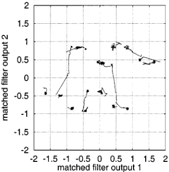
To illustrate the optimal properties of the enhanced -means clustering method, consider the user 2 of Example 1 given in the previous section with SNR SNR dB. Started
from , , the trajectories of cluster
cen-ters in 10 000-samples adaptation are shown in Fig. 8. Table V summarizes the final cluster center positions and variations, in comparison with the true noise-free signal states. Similar clus-tering performance can be obtained with only 4000 data samples when the first 16 data points are used as the initial centers, as illustrated in Fig. 9. The BER performance of such a clustering RBF MUD is indistinguishable with the optimal one-shot MUD. The following comparisons for the SVM and clustering RBF MUDs can be made. The adaptation of the SVM model is based on a block of data while the clustering RBF is implemented sample-by-sample. The sample-by-sample adjustment is more desired in real-time applications. The clustering RBF MUD can achieve the optimal MUD, provided that a sufficient number of training data are available. The SVM MUD has an important advantage as it requires a relatively short training data set. For our simple Example 1, The SVM MUD requires less than 200 training data. In contrast, the clustering RBF MUD needs a few thousands of training data, due to the nature of the unsupervised clustering process. Such a long training data length is difficult to achieve in practice. As the SVM approach places the kernel centers directly on some noisy data points called SVs, it will re-quire more centers than the clustering RBF model. For Example 1, the SVM MUD needs typically 40 kernels to closely match the optimal performance, while the clustering RBF MUD has only 16 kernel functions.
VII. CONCLUSION
Fig. 8. Cluster center trajectories using the enhanced-means clustering for user 2 of Example 1. SNR = SNR = 20 dB, initial centers are all placed at the origin, and 10 000 data samples are used.
TABLE V
CLUSTERCENTERS ANDVARIATIONSOBTAINEDUSING THEENHANCED
-MEANSCLUSTERING FORUSER2OFEXAMPLE1. SNR = SNR = 20 dB (NOISEVARIANCE0.001), INITIALCENTERSAREALLPLACED AT THE
ORIGIN,AND10 000 DATASAMPLESAREUSED
APPENDIX
During one bit period, the chip rate sampler produces sam-ples
(38)
The baseband model for is represented by [36]
. .. ... ..
. . .. . .. ...
.. .
(39)
Fig. 9. Cluster center trajectories using the enhanced-means clustering for user 2 of Example 1. SNR = SNR = 20 dB, the first 16 data points are used as initial centers, and 4000 data samples are used.
where the system matrix is defined as
. .. ... ..
. . .. . ..
(40)
An MUD can directly operate on , instead of the chip-matched filtered version . For example, an alternative linear MUD takes the form
(41)
with the -dimensional weight vector .
It is well-known that this linear MUD is equivalent to the linear MUD of (13). In the -dimensional space , the set of the
noise-free received signal states is defined by
(42)
An optimal Bayesian one-shot detector, similar to (21), can al-ternatively be defined.
REFERENCES
[1] R. Prasad, CDMA for Wireless Personal Communications. Norwood, MA: Artech House, 1996.
[2] S. Verdú, “Minimum probability of error for asynchronous Gaussian multiple-access channels,” IEEE Trans. Inform. Theory, vol. IT-32, pp. 85–96, 1986.
[3] S. Moshavi, “Multiuser detection for DS-CDMA communications,”
IEEE Commun. Mag., vol. 34, no. 10, pp. 124–136, 1996.
[4] S. Verdú, Multiuser Detection. Cambridge, U.K.: Cambridge Univ. Press, 1998.
[5] Z. Xie, R. T. Short, and C. K. Rushforth, “A family of suboptimum de-tectors for coherent multiuser communications,” IEEE J. Select. Areas
Commun., vol. 8, pp. 683–690, 1990.
[6] U. Madhow and M. L. Honig, “MMSE interference suppression for di-rect-sequence spread-spectrum CDMA,” IEEE Trans. Commun., vol. 42, pp. 3178–3188, 1994.
[7] S. L. Miller, “An adaptive direct-sequence code-division multiple-access receiver for multiuser interference rejection,” IEEE Trans. Commun., vol. 43, pp. 1746–1755, 1995.
[image:7.612.343.510.62.232.2][9] G. Woodward and B. S. Vucetic, “Adaptive detection for DS-CDMA,”
Proc. IEEE, vol. 86, no. 7, pp. 1413–1434, 1998.
[10] N. B. Mandayam and B. Aazhang, “Gradient estimation for sensitivity analysis and adaptive multiuser interference rejection in code-division multi-access systems,” IEEE Trans. Commun., vol. 45, no. 7, pp. 848–858, 1997.
[11] X. F. Wang, W. S. Lu, and A. Antoniou, “Constrained minimum-BER multiuser detection,” in Proc. ICASSP, vol. 5, Phoenix, AZ, May 14–18, 1999, pp. 2603–2606.
[12] I. N. Psaromiligkos, S. N. Batalama, and D. A. Pados, “On adaptive min-imum probability of error linear filter receivers for DS-CDMA chan-nels,” IEEE Trans. Commun., vol. 47, no. 7, pp. 1092–1102, 1999. [13] C. C. Yeh, R. R. Lopes, and J. R. Barry, “Approximate minimum
bit-error rate multiuser detection,” in Proc. Globecom’98, Sydney, Aus-tralia, Nov. 1998, pp. 3590–3595.
[14] S. Chen, A. K. Samingan, B. Mulgrew, and L. Hanzo, “Adaptive min-imum-BER linear multiuser detection for DS-CDMA signals in multi-path channels,” IEEE Trans. Signal Processing, June 2001, to be pub-lished.
[15] B. Aazhang, B. P. Paris, and G. C. Orsak, “Neural networks for multiuser detection in code-division multiple-access communications,”
IEEE Trans. Commun., vol. 40, pp. 1212–1222, 1992.
[16] U. Mitra and H. V. Poor, “Neural network techniques for adaptive multiuser demodulation,” IEEE J. Select. Areas Commun., vol. 12, pp. 1460–1470, 1994.
[17] D. G. M. Cruickshank, “Radial basis function receivers for DS-CDMA,”
Electron. Lett., vol. 32, no. 3, pp. 188–190, 1996.
[18] R. Tanner and D. G. M. Cruickshank, “Volterra based receivers for DS-CDMA,” in Proc. 8th IEEE Int. Symp. Personal, Indoor, Mobile
Radio Commun., vol. 3, September 1997, pp. 1166–1170.
[19] V. Vapnik, The Nature of Statistical Learning Theory. New York: Springer-Verlag, 1995.
[20] B. Schölkopf, K. K. Sung, C. J. C. Burges, F. Girosi, P. Niyogi, T. Poggio, and V. Vapnik, “Comparing support vector machines with Gaussian ker-nels to radial basis function classifiers,” IEEE Trans. Signal Processing, vol. 45, pp. 2758–2765, 1997.
[21] C. J. C. Burges, “A tutorial on support vector machines for pattern recognition,” Data Mining and Knowledge Discovery, vol. 2, no. 2, pp. 121–167, 1998.
[22] V. Vapnik, “The support vector method of function estimation,” in
Non-linear Modeling: Advanced Black-Box Techniques, J. A. K. Suykens and
J. Vandewalle, Eds. Boston, MA: Kluwer, 1998, pp. 55–85. [23] J. Platt, “Fast training of support vector machines using sequential
minimal optimization,” in Advances in Kernel Methods—Support
Vector Learning, B. Schölkopf, C. J. C. Burges, and A. J. Smola,
Eds. Cambridge, MA: MIT Press, 1999, pp. 185–208.
[24] “Special Issue on VC Learning Theory and Its Applications,” IEEE
Trans. Neural Networks, vol. 10, no. 5, Sept. 1999.
[25] A. Lyhyaoui, M. Martínez, I. Mora, M. Vázquez, J. L. Sancho, and A. R. Figueiras-Vidal, “Sample selection via clustering to construct sup-port vector-like classifiers,” IEEE Trans. Neural Networks, vol. 10, pp. 1474–1481, 1999.
[26] N. Cristianini and J. Shawe-Taylor, An Introduction to Support Vector
Machines. Cambridge, U.K.: Cambridge Univ. Press, 2000. [27] S. Chen, S. Gunn, and C. J. Harris, “Decision feedback equalizer design
using support vector machines,” Inst. Elect. Eng. Proc. Vision, Image
and Signal Processing, vol. 147, no. 3, pp. 213–219, 2000.
[28] D. J. Sebald and J. A. Bucklew, “Support vector machine techniques for nonlinear equalization,” IEEE Trans. Signal Processing, vol. 48, pp. 3217–3226, 2000.
[29] F. Albu and D. Martinez, “The application of support vector machines with Gaussian kernels for overcoming co-channel interference,” in
Proc. 9th IEEE Int. Workshop Neural Networks for Signal Processing,
Madison, WI, Aug. 23–25, 1999, pp. 49–57.
[30] F. Pérez-Cruz, A. Navia-Vázquez, P. L. Alarcón-Diana, and A. Artés-Rodríguez, “SVC-based equalizer for burst TDMA transmis-sion,” Signal Processing, 2000.
[31] S. Chen, B. Mulgrew, and P. M. Grant, “A clustering technique for dig-ital communications channel equalization using radial basis function networks,” IEEE Trans. Neural Networks, vol. 4, pp. 570–579, 1993. [32] S. Chen, “Nonlinear time series modeling and prediction using Gaussian
RBF networks with enhanced clustering and RLS learning,” Electron.
Lett., vol. 31, no. 2, pp. 117–118, 1995.
[33] C. Chinrungrueng and C. H. Séquin, “Optimal adaptive-means algo-rithm with dynamic adjustment of learning rate,” IEEE Trans. Neural
Networks, vol. 6, pp. 157–169, 1995.
[34] S. Chen, S. McLaughlin, B. Mulgrew, and P. M. Grant, “Bayesian de-cision feedback equaliser for overcoming cochannel interference,” Inst.
Elect. Eng. Proc. Commun., vol. 143, no. 4, pp. 219–225, 1996.
[35] P. P. Vaidyanathan, Multirate Systems and Filter Banks. Englewood Cliffs, NJ: Prentice-Hall, 1993.
[36] B. Mulgrew, “Nonlinear signal processing for adaptive equalization and multi-user detection,” in Proc. EUSIPCO 98, Rhodes, Greece, Sept. 1998, pp. 537–544.
[37] S. S. Keerthi, S. K. Shevade, C. Bhattacharyya, and K. R. K. Murthy, “A fast iterative nearest point algorithm for support vector machine classi-fier design,” Intell. Syst. Lab, Dept. Comput.Sci. Automation, Indian Institute of Science, Tech. Rep. TR-ISL-99-03, 1999.