Do Supervised Distributional Methods Really Learn Lexical Inference Relations?

Do Supervised Distributional Methods

Really Learn Lexical Inference Relations?

Omer Levy† _{Steffen Remus}§ _{Chris Biemann}§ _{Ido Dagan}†

†Natural Language Processing Lab §Language Technology Lab

Bar-Ilan University Technische Universität Darmstadt

Ramat-Gan, Israel Darmstadt, Germany

{omerlevy,dagan}@cs.biu.ac.il {remus,biem}@cs.tu-darmstadt.de

Abstract

Distributional representations of words have been recently used in supervised settings for recognizing lexical inference relations be-tween word pairs, such as hypernymy and en-tailment. We investigate a collection of these state-of-the-art methods, and show that they do not actually learn a relation between two words. Instead, they learn an independent property of a single word in the pair: whether that word is a “prototypical hypernym”.

1 Introduction

Inference in language involves recognizing infer-ence relations between two words (x and y), such as causality (flu → fever), hypernymy (cat → animal), and other notions of lexical entailment. The distributional approach to automatically recog-nize these relations relies on representing each word x as a vector~xofcontextual features: other words that tend to appear in its vicinity. Such features are typically used in word similarity tasks, where cosine similarity is a standard similarity measure between two word vectors:sim(x, y) =cos(~x, ~y).

Many unsupervised distributional methods of rec-ognizing lexical inference replace cosine similarity with an asymmetric similarity function (Weeds and Weir, 2003; Clarke, 2009; Kotlerman et al., 2010; Santus et al., 2014). Supervised methods, reported to perform better, try to learn the asymmetric opera-tor from a training set. The various supervised meth-ods differ by the way they represent each candidate pair of words(x, y): Baroni et al. (2012) use con-catenation~x⊕~y, others (Roller et al., 2014; Weeds

et al., 2014; Fu et al., 2014) take the vectors’ differ-ence~y−~x, and more sophisticated representations, based on contextual features, have also been tested (Turney and Mohammad, 2014; Rimell, 2014).

In this paper, we argue that these supervised meth-ods do not, in fact, learn to recognize lexical infer-ence. Our experiments reveal that much of their pre-viously perceived success stems from lexical mem-orizing. Further experiments show that these super-vised methods learn whetheryis a “prototypical hy-pernym” (i.e. a category), regardless of x, rather than learning a concrete relation betweenxandy.

Our mathematical analysis reveals that said meth-ods ignore the interaction betweenxandy, explain-ing our empirical findexplain-ings. We modify them ac-cordingly by incorporating the similarity between x and y. Unfortunately, the improvement in per-formance is incremental. We suspect that methods based solely on contextual features of single words are not learning lexical inference relations because contextual features might lack the necessary infor-mation to deduce how one word relates to another.

2 Experiment Setup

Due to various differences (e.g. corpora, train/test splits), we do not list previously reported results, but apply a large space of state-of-the-art supervised methods and review them comparatively. We ob-serve similar trends to previously published results, and make the dataset splits available for replication.1

1_{http://u.cs.biu.ac.il/~nlp/resources/} downloads/

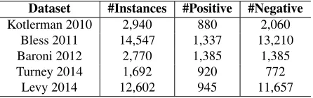
Dataset #Instances #Positive #Negative

Kotlerman 2010 2,940 880 2,060

Bless 2011 14,547 1,337 13,210

Baroni 2012 2,770 1,385 1,385

Turney 2014 1,692 920 772

Levy 2014 12,602 945 11,657

Table 1: Datasets evaluated in this work.

2.1 Word Representations

We built 9 word representations over Wikipedia (1.5 billion tokens) using the cross-product of 3 types of contexts and 3 representation models.

2.1.1 Context Types

Bag-of-WordsUses 5 tokens to each side of the tar-get word (10 context words in total). It also employs subsampling (Mikolov et al., 2013a) to increase the impact of content words.

Positional Uses only 2 tokens to each side of the target word, and decorates them with their position (relative to the target word); e.g.the−1is a common

positional context ofcat(Schütze, 1993).

Dependency Takes all words that share a syntactic connection with the target word (Lin, 1998; Padó and Lapata, 2007; Baroni and Lenci, 2010). We used the same parsing apparatus as in (Levy and Gold-berg, 2014).

2.1.2 Representation Models

PPMIA word-context positive pointwise mutual in-formation matrixM (Niwa and Nitta, 1994).

SVD We reduced M’s dimensionality to k= 500

using Singular Value Decomposition (SVD).2

SGNSSkip-grams with negative sampling (Mikolov et al., 2013b) with 500 dimensions and 5 nega-tive samples. SGNS was trained using a modified version ofword2vecthat allows different context types (Levy and Goldberg, 2014).3

2.2 Labeled Datasets

We used 5 labeled datasets for evaluation. Each dataset entry contains two words(x, y) and a label whetherxentailsy. Note that each dataset was cre-ated with a slightly different goal in mind, affecting word-pair generation and annotation. For example, 2_{Following Caron (2001), we used the square root of the} eigenvalue matrixΣkfor representing words:Mk=Uk√Σk.

3_{http://bitbucket.org/yoavgo/word2vecf}

both of Baroni’s datasets are designed to capture hy-pernyms, while other datasets try to capture broader notions of lexical inference (e.g. causality). Table 1 provides metadata on each dataset, and the descrip-tion below explains how each one was created.

(Kotlerman et al., 2010)Manually annotated lexi-cal entailment of distributionally similar nouns.

(Baroni and Lenci, 2011) a.k.a. BLESS. Created by selecting unambiguous word pairs and their se-mantic relations from WordNet. Following Roller et al. (2014), we labeled noun hypernyms as positive examples and used meronyms, noun cohyponyms, and random noun pairs as negative.

(Baroni et al., 2012) Created in a similar fashion to BLESS. Hypernym pairs were selected as posi-tive examples from WordNet, and then permutated to generate negative examples.

(Turney and Mohammad, 2014) Based on a crowdsourced dataset of 79 semantic relations (Ju-rgens et al., 2012). Each semantic relation was lin-guistically annotated as entailing or not.

(Levy et al., 2014) Based on manually anno-tated entailment graphs of subject-verb-object tuples (propositions). Noun entailments were extracted from entailing tuples that were identical except for one of the arguments, thus propagating the exis-tence/absence of proposition-level entailment to the noun level. This dataset is the most realistic dataset, since the original entailment annotations were made in the context of a complete proposition.

2.3 Supervised Methods

We tested 4 compositions for representing(x, y)as a feature vector:concat(~x⊕~y) (Baroni et al., 2012),

diff(~y−~x) (Roller et al., 2014; Weeds et al., 2014; Fu et al., 2014),only x(~x), andonly y(~y). For each composition, we trained two types of classifiers, tun-ing hyperparameters with a validation set: logistic regression withL1 or L2 regularization, and SVM

with a linear kernel or quadratic kernel.

3 Negative Results

exper-Dataset Lexical +Contextual ∆

Kotlerman 2010 .346 .437 .091

Bless 2011 .960 .960 .000

Baroni 2012 .638 .802 .164

Turney 2014 .644 .747 .103

Levy 2014 .302 .370 .068

Table 2: The performance (F1) of lexical versus contex-tual feature classifiers on a random train/test split with lexical overlap.

iments by applying the JoBimText framework4 _for

scalable distributional thesauri (Biemann and Riedl, 2013) using Google’s syntactic N-grams (Goldberg and Orwant, 2013) as a corpus.

Lexical Memorization is the phenomenon in which the classifier learns that a specific word in a specific slot is a strong indicator of the label. For example, if a classifier sees many positive examples wherey = animal, it may learn that anything that appears with y = animal is likely to be positive, effectivelymemorizingthe wordanimal.

The following experiment shows that supervised methods with contextual features are indeed mem-orizing words from the training set. We randomly split each dataset into70%train,5%validation, and

25%test, and train lexical-feature classifiers, using a one-hot vector representation ofyas input features. By definition, these classifiers memorize words from the training set. We then add contextual-features (as described in §2.1), on top of the lexical features, and train classifiers analogously. Table 2 compares the best lexical- and contextual-feature classifiers on each dataset. The performance difference is under 10 points in the larger datasets, showing that much of the contextual-feature classifiers’ success is due to lexical memorization. Similar findings were also reported by Roller et al. (2014) and Weeds et al. (2014), supporting our memorization argument.

To prevent lexical memorization in our following experiments, we split each dataset into train and test sets with zero lexical overlap. We do this by ran-domly splitting the vocabulary into “train” and “test” words, and extract train-only and test-only subsets of each dataset accordingly. About half of each original dataset contains “mixed” examples (one train-word and one test-word); these are discarded.

4_{http://jobimtext.org}

Dataset Best Supervised Only~y Unsupervised

Kotlerman 2010 .408 .375 .461

Bless 2011 .665 .637 .197 Baroni 2012 .774 .663 .788

Turney 2014 .696 .649 .642 Levy 2014 .324 .324 .231

Table 3: A comparison of each dataset’s best supervised method with: (a) the best result usingonly y composi-tion; (b) unsupervised cosine similaritycos(~x, ~y). Perfor-mance is measured byF1. Uses lexical train/test splits.

Supervised vs Unsupervised While supervised methods were reported to perform better than un-supervised ones, this is not always the case. As a baseline, we measured the “vanilla” cosine similar-ity ofxandy, tuning a threshold with the validation set. This unsupervised symmetric method outper-forms all supervised methods in 2 out of 5 datasets (Table 3).

Ignoringx’s Information We compared the per-formance ofonly yto that of the best configuration in each dataset (Table 3). In 4 out of 5 datasets, the difference in performance is less than 5 points. This means that the classifiers areignoring most of the information inx. Furthermore, they might be over-looking the compatibility (or incompatibility) ofxto y. Weeds et al. (2014) reported a similar result, but did not address the fundamental question it beckons: if the classifiercannotcapture a relation betweenx andy, then what is it learning?

4 Prototypical Hypernyms

We hypothesize that the supervised methods exam-ined in this paper are learning whethery is a likely “category” word – a prototypical hypernym– and, to a lesser extent, whether x is a likely “instance” word. This hypothesis is consistent with our previ-ous observations (§3).

Though the terms “instance” and “category” per-tain to hypernymy, we use them here in the broader sense of entailment, i.e. as “tends to entail” and “tends to be entailed”, respectively. We later show (§4.2) that this phenomenon indeed extends to other inference relations, such as meronymy.

4.1 Testing the Hypothesis

instance-Dataset Top Positional Contexts ofy

Kotlerman 2010 grave−1,substances+2,lend-lease−1,poor−2,bureaucratic−1,physical−1,dry−1,air−1,civil−1 Bless 2011 other−1,resembling+1,such+1,assemblages+1,magical−1,species+1,any−2,invertebrate−1 Baroni 2012 any−1,any−2,social−1,every−1,this−1,kinds−2,exotic−1,magical−1,institute−2,important−1 Turney 2014 of+1,inner−1,including+1,such+1,considerable−1,their−1,extra−1,types−2,different−1,other−1

Levy 2014 psychosomatic−1,unidentified−1,auto-immune+2,specific−1,unspecified−1,treatable−2,any−1

Table 4: Top positional features learned with logistic regression overconcat. Displaying positive features ofy.

category pairs, e.g. (banana, animal). For each dataset, we generate a set of such synthetic exam-plesS, by taking the positive examples from the test portionT+_{, and extracting all of its instance words}

T+

x and category wordsTy+.

T_x+={x|(x, y)∈T+} T_y+ ={y|(x, y)∈T+}

We then defineSas all the in-place combinations of instance-category word pairs that did not appear in T+_{, and are therefore likely to be false.}

S= T_x+×T_y+\T+

Finally, we test the classifier on a sample ofS(due to its size). Since all examples are assumed to be false, we measure the false positive rate as match error

– the error of classifying a mismatching instance-category pair as positive.

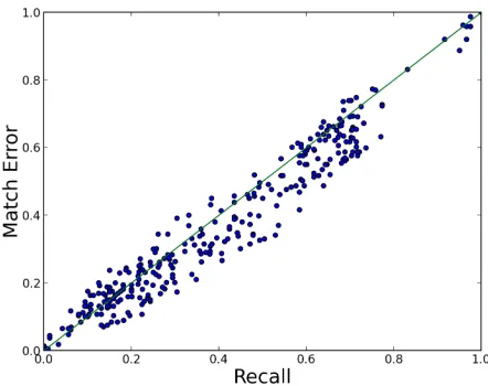
According to our hypothesis, the classifier can-not differentiate between matched and mismatched examples (T+ _{and S, respectively). We therefore}

expect it to classify a similar proportion ofT+ _and

S as positive. We validate this by comparingrecall

(proportion ofT+_{classified as positive) tomatch} er-ror(proportion ofSclassified as positive). Figure 1 plots these two measures across all configurations and datasets, and finds them to be extremely close (regression curve: match error = 0.935·recall), thus confirming our hypothesis.

4.2 Prototypical Hypernym Features

A qualitative way of analyzing our hypothesis is to look at which features the classifiers tend to con-sider. Since SVD and SGNS features are not eas-ily interpretable, we used PPMI with positional con-texts as our representation, and trained a logistic re-gression model withL1regularization usingconcat

over the entire dataset (no splits). We then observed the features with the highest weights (Table 4).

Figure 1: The correlation of recall (positive rate onT+₎ with match error (positive rate onS) compared to perfect correlation (green line).

Many of these features describe dataset-specific category words. For example, in Levy’s medical-domain dataset, many words entail “symptom”, which is captured by the discriminative feature psychosomatic−1. Other features are

domain-independent indicators of category, e.g. any−1,

every−1, andkinds−2. The most striking features,

though, are those that occur in Hearst (1992) pat-terns: other−1, such+1, including+1, etc. These

features appear in all datasets, and their analogues are often observed forx(e.g. such−2). Even

quali-tatively, many of the dominant features capture pro-totypical or dataset-specific hypernyms.

As mentioned, the datasets examined in this work also contain inference relations other than hyper-nymy. In Turney’s dataset, for example, 77 % of positive pairs are non-hypernyms, and y is of-ten a quality (coat → warmth) or a component (chair → legs) of x. Qualities and components can often be detected via possessives, e.g.of+1and

andexotic−1, may also indicate qualities. These

ex-amples suggest that our hypothesis extends beyond hypernymy to other inference relations as well. 5 Analysis of Vector Composition

Our empirical findings show thatconcatanddiffare clearly ignoring the relation betweenxandy. To un-derstand why, we analyze these compositions in the setting of a linear SVM. Given a test example,(x, y)

and a training example that is part of the SVM’s sup-port(xs, ys), the linear kernel function yields

Equa-tions (1) forconcatand (2) fordiff.

K(~x⊕~y, ~xs⊕~ys) =~x·x~s+~y·~ys (1)

K(~y−~x, ~ys−x~s) =~x·x~s+~y·~ys−~x·~ys−~y·x~s (2)

Assuming all vectors are normalized (as in our ex-periments), the kernel function ofconcatis actually the similarity of the x-words plus the similarity of they-words. Two dis-similarity terms are added to

diff’s kernel, preventing thexof one pair from being too similar to the other pair’sy(and vice versa).

Notice the absence of the term~x·~y. This means that the classifier has no way of knowing ifxandy are even related, let alone entailing. This flaw makes the classifier believe that any instance-category pair

(x, y) is in an entailment relation, even if they are unrelated, as seen in §4. Polynomial kernels also lack~x·~y, and thus suffer from the same flaw. 6 Adding Intra-Pair Similarity

Using an RBF kernel withdiffslightly mitigates this issue, as it factors in~x·~y, among other similarities:

KRBF(~y−~x, ~ys−x~s) =e−σ12|(~y−~x)−(y~s−x~s)|2

=e−σ12(~x~y+x~sy~s+~x ~xs+~y ~ys−~x ~ys−~y ~xs−2) (3) A more direct approach of incorporating~x·~yis to create a new kernel, which balances intra-pair simi-larities with inter-pair ones:

KSIM((~x, ~y),(x~s, ~ys)) = (~x~y·x~s~ys)α2(~x ~x_s·~y ~y_s)1−2α (4)

While these methods reduce match error – match error = 0.618·recallversus the previous regression curve ofmatch error = 0.935·recall – their overall performance is only incrementally better than that of linear methods (Table 5). This improvement is also, partially, a result of the non-linearity introduced in these kernels.

Dataset LIN(concat) LIN(diff) RBF(diff) SIM

Kotlerman 2010 .367 .187 .407 .332 Bless 2011 .634 .665 .636 .687

Baroni 2012 .745 .769 .848 .859

Turney 2014 .696 .694 .691 .641 Levy 2014 .229 .219 .252 .244

Table 5: Performance (F1) of SVM across kernels. LIN refers to the linear kernel (equations (1) and (2)),RBFto the Gaussian kernel (equation (3)), andSIMto our new kernel (equation (4)). Uses lexical train/test splits.

7 The Limitations of Contextual Features

In this work, we showed that state-of-the-art su-pervised methods for recognizing lexical inference appear to be learning whether y is a prototypical hypernym, regardless of its relation with x. We tried to factor in the similarity between x and y, yet observed only marginal improvements. While more sophisticated methods might be able to extract the necessary relational information from contextual features alone, it is also possible that this informa-tion simplydoes not existin those features.

A (de)motivating example can be seen in §4.2. A typicaly often has such+1 as a dominant feature,

whereasxtends to appear withsuch−2. These

fea-tures are relics of the Hearst (1992) pattern “ysuch asx”. However, contextual features of single words cannot capture thejointoccurrence ofxandyin that pattern; instead, they record only this observation as two independent features of different words. In that sense, contextual features are inherently hand-icapped in capturing relational information, requir-ing supervised methods to harness complementary information from more sophisticated features, such as textual patterns that connectxwithy(Snow et al., 2005; Turney, 2006).

Acknowledgements

References

Marco Baroni and Alessandro Lenci. 2010. Distribu-tional memory: A general framework for corpus-based semantics. Computational Linguistics, 36(4):673– 721.

Marco Baroni and Alessandro Lenci. 2011. How we blessed distributional semantic evaluation. In Pro-ceedings of the GEMS 2011 Workshop on GEometrical Models of Natural Language Semantics, pages 1–10, Edinburgh, UK.

Marco Baroni, Raffaella Bernardi, Ngoc-Quynh Do, and Chung-chieh Shan. 2012. Entailment above the word level in distributional semantics. InProceedings of the 13th Conference of the European Chapter of the As-sociation for Computational Linguistics, pages 23–32, Avignon, France.

Chris Biemann and Martin Riedl. 2013. Text: Now in 2D! A framework for lexical expansion with con-textual similarity. Journal of Language Modelling, 1(1):55–95.

John Caron. 2001. Experiments with LSA scor-ing: Optimal rank and basis. In Proceedings of the SIAM Computational Information Retrieval Work-shop, pages 157–169.

Daoud Clarke. 2009. Context-theoretic semantics for natural language: an overview. In Proceedings of the Workshop on Geometrical Models of Natural Lan-guage Semantics, pages 112–119, Athens, Greece. Ruiji Fu, Jiang Guo, Bing Qin, Wanxiang Che, Haifeng

Wang, and Ting Liu. 2014. Learning semantic hier-archies via word embeddings. InProceedings of the 52nd Annual Meeting of the Association for Compu-tational Linguistics (Volume 1: Long Papers), pages 1199–1209, Baltimore, Maryland.

Yoav Goldberg and Jon Orwant. 2013. A dataset of syntactic-ngrams over time from a very large corpus of english books. InSecond Joint Conference on Lex-ical and Computational Semantics (*SEM), Volume 1: Proceedings of the Main Conference and the Shared Task: Semantic Textual Similarity, pages 241–247, At-lanta, Georgia, USA.

Marti A Hearst. 1992. Automatic acquisition of hy-ponyms from large text corpora. In COLING 1992 Volume 2: The 15th International Conference on Computational Linguistics, pages 529–545, Nantes, France.

David A Jurgens, Peter D Turney, Saif M Mohammad, and Keith J Holyoak. 2012. Semeval-2012 task 2: Measuring degrees of relational similarity. In *SEM 2012: The First Joint Conference on Lexical and Com-putational Semantics – Volume 1: Proceedings of the main conference and the shared task, and Volume 2: Proceedings of the Sixth International Workshop on

Semantic Evaluation (SemEval 2012), pages 356–364, Montréal, Quebec, Canada.

Lili Kotlerman, Ido Dagan, Idan Szpektor, and Maayan Zhitomirsky-Geffet. 2010. Directional distributional similarity for lexical inference. Natural Language En-gineering, 4(16):359–389.

Omer Levy and Yoav Goldberg. 2014. Dependency-based word embeddings. InProceedings of the 52nd Annual Meeting of the Association for Computational Linguistics (Volume 2: Short Papers), pages 302–308, Baltimore, Maryland.

Omer Levy, Ido Dagan, and Jacob Goldberger. 2014. Focused entailment graphs for open ie propositions. InProceedings of the Eighteenth Conference on Com-putational Natural Language Learning, pages 87–97, Baltimore, Maryland.

Dekang Lin. 1998. Automatic retrieval and clustering of similar words. InProceedings of the 36th Annual Meeting of the Association for Computational Linguis-tics and 17th International Conference on Computa-tional Linguistics, Volume 2, pages 768–774, Mon-tréal, Quebec, Canada.

Tomas Mikolov, Kai Chen, Greg Corrado, and Jeffrey Dean. 2013a. Efficient estimation of word repre-sentations in vector space. In Proceedings of the In-ternational Conference on Learning Representations (ICLR).

Tomas Mikolov, Ilya Sutskever, Kai Chen, Gregory S Corrado, and Jeffrey Dean. 2013b. Distributed rep-resentations of words and phrases and their composi-tionality. InAdvances in Neural Information Process-ing Systems, pages 3111–3119.

Yoshiki Niwa and Yoshihiko Nitta. 1994. Co-occurrence vectors from corpora vs. distance vectors from dictio-naries. InCOLING 1994 Volume 1: The 15th Interna-tional Conference on ComputaInterna-tional Linguistics, Ky-oto, Japan.

Sebastian Padó and Mirella Lapata. 2007. Dependency-based construction of semantic space models. Compu-tational Linguistics, 33(2):161–199.

Laura Rimell. 2014. Distributional lexical entailment by topic coherence. InProceedings of the 14th Confer-ence of the European Chapter of the Association for Computational Linguistics, pages 511–519, Gothen-burg, Sweden.

Stephen Roller, Katrin Erk, and Gemma Boleda. 2014. Inclusive yet selective: Supervised distributional hy-pernymy detection. In Proceedings of COLING 2014, the 25th International Conference on Compu-tational Linguistics: Technical Papers, pages 1025– 1036, Dublin, Ireland.

Conference of the European Chapter of the Associa-tion for ComputaAssocia-tional Linguistics, volume 2: Short Papers, pages 38–42, Gothenburg, Sweden.

Hinrich Schütze. 1993. Part-of-speech induction from scratch. InProceedings of the 31st Annual Meeting of the Association for Computational Linguistics, pages 251–258, Columbus, Ohio, USA.

Rion Snow, Daniel Jurafsky, and Andrew Y Ng. 2005. Learning syntactic patterns for automatic hypernym discovery. In Advances in Neural Information Pro-cessing.

Peter D Turney and Saif M Mohammad. 2014. Experi-ments with three approaches to recognizing lexical en-tailment.Natural Language Engineering, pages 1–40. Peter D Turney. 2006. Similarity of semantic relations.

Computational Linguistics, 32(3):379–416.

Julie Weeds and David Weir. 2003. A general frame-work for distributional similarity. In Proceedings of the 2003 Conference on Empirical Methods in Natural Language Processing, pages 81–88, Sapporo, Japan. Julie Weeds, Daoud Clarke, Jeremy Reffin, David Weir,