A New Parsing Algorithm for Combinatory Categorial Grammar
Marco Kuhlmann Department of
Computer and Information Science Linköping University, Sweden marco.kuhlmann@liu.se
Giorgio Satta Department of Information Engineering University of Padua, Italy satta@dei.unipd.it
Abstract
We present a polynomial-time parsing algo-rithm for CCG, based on a new decomposition of derivations into small, shareable parts. Our algorithm has the same asymptotic complex-ity,O.n6/, as a previous algorithm by
Vijay-Shanker and Weir (1993), but is easier to un-derstand, implement, and prove correct.
1 Introduction
Combinatory Categorial Grammar (CCG; Steedman and Baldridge (2011)) is a lexicalized grammar for-malism that belongs to the class of so-called mildly context-sensitive formalisms, as characterized by Joshi (1985). CCG has been successfully used for a wide range of practical tasks including data-driven parsing (Clark and Curran, 2007), wide-coverage se-mantic construction (Bos et al., 2004; Kwiatkowski et al., 2010; Lewis and Steedman, 2013) and machine translation (Weese et al., 2012).
Several parsing algorithms for CCG have been presented in the literature. Earlier proposals show running time exponential in the length of the input string (Pareschi and Steedman, 1987; Tomita, 1988). A breakthrough came with the work of Vijay-Shanker and Weir (1990) and Vijay-Shanker and Weir (1993) who report the first polynomial-time algorithm for CCG parsing. Until this day, this algorithm, which we shall refer to as the V&W algorithm, remains the
onlypublished polynomial-time parsing algorithm for CCG. However, we are not aware of any practical parser for CCG that actually uses it. We speculate that this has two main reasons: First, some authors
have argued that linguistic resources available for CCG can be covered with context-free fragments of the formalism (Fowler and Penn, 2010), for which more efficient parsing algorithms can be given. Sec-ond, the V&W algorithm is considerably more com-plex than parsing algorithms for equivalent mildly context-sensitive formalisms, such as Tree-Adjoin-ing Grammar (Joshi and Schabes, 1997), and is quite hard to understand, implement, and prove correct.
The V&W algorithm is based on a special decom-position of CCG derivations into smaller parts that can then be shared among different derivations. This sharing is the key to the polynomial runtime. In this article we build on the same idea, but develop an alternative polynomial-time algorithm for CCG parsing. The new algorithm is based on a different decomposition of CCG derivations, and is arguably simpler than the V&W algorithm in at least two re-spects: First, the new algorithm uses only three basic steps, against the nine basic steps of the V&W parser. Second, the correctness proof of the new algorithm is simpler than the one reported by Vijay-Shanker and Weir (1993). The new algorithm runs in timeO.n6/ wherenis the length of the input string, the same as the V&W parser.
We organize our presentation as follows. In Sec-tion 2 we introduce CCG and the central noSec-tion of derivation trees. In Section 3 we start with a simple but exponential-time parser for CCG, from which we derive our polynomial-time parser in Section 4. Section 5 further simplifies the algorithm and proves its correctness. We then provide a discussion of our algorithm and possible extensions in Section 6. Sec-tion 7 concludes the article.
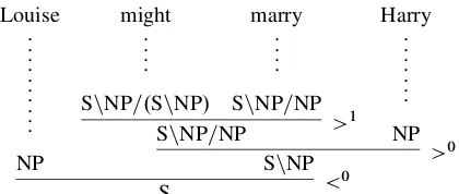
2 Combinatory Categorial Grammar We assume basic familiarity with CCG in general and the formalism of Weir and Joshi (1988) in particular. In this section we set up our terminology and notation. A CCG has two main parts: alexiconthat associates words with categories, and rules that specify how categories can be combined into other categories. Together, these components give rise toderivations
such as the one shown in Figure 1.
2.1 Lexicon
The CCG lexicon is a finite set of word–category pairs w WD X.1 Categories are built from a finite set ofatomic categoriesand two binary operators: forward slash (=) and backward slash ( = ). Atomic categories represent the syntactic types of complete constituents; they include a distinguished categoryS for complete sentences. A constituent with the com-plex categoryX =Y represents a function that seeks a constituent of categoryY immediately to its right and returns a constituent of categoryX; similarly,X = Y represents a function that seeks aY to its left. We treat slashes as left-associative operators and omit unnecessary parentheses. By this convention, every categoryX can be written as
X DAjmXm j1X1
where m 0, A is an atomic category called the
target of X and the jiXi are slash–category pairs
called theargumentsofX. We view these arguments as being arranged in a stack withj1X1at the top and
jmXm at the bottom. Thus another way of writing
the categoryX above is asX D A˛, where˛ is a (possibly empty) stack ofmarguments. The number mis called thearityofX; we denote it byar.X /.
2.2 Rules
The rules of CCG are directed versions of (general-ized) functional composition. There are two forms,
forward rulesandbackward rules:
X =Y YjdYd j1Y1)XjdYd j1Y1 .>d/
YjdYd j1Y1 X = Y )XjdYd j1Y1 .<d/
1The formalism of Weir and Joshi (1988) also allows lexicon
entries for the empty string, a feature that we ignore here.
Louise .. .. .. .. .. NP
might .. .. S = NP=.S = NP/
marry .. .. S = NP=NP
S = NP=NP >1
Harry .. .. .. . NP
S = NP >
0
[image:2.612.322.532.53.142.2]S <0
Figure 1: A sample derivation tree.
Every rule is obtained by choosing a specificdegree
d 0and specific directions (forward or backward) for each of the slashes ji, whileX, Y and the Yi
are variables ranging over categories. Thus for every degree d 0 there are 2d forward rules and2d backward rules. The rules of degree0 are called
applicationrules. In contexts where we refer to both application and composition, we use the latter term for “proper” composition rules of degree d > 0. Note that in most of this article we ignore additional rules required for linguistic analysis with CCG, in particular type-raising and substitution. We briefly discuss these rules in Section 6.
Every CCG grammar restricts itself to a finite set of rules, but each such rule may give rise to infinitely manyrule instances. A rule is instantiated by sub-stituting concrete categories for the variables. For example, the derivation in Figure 1 contains the fol-lowing instance of forward composition (>1):
S = NP=.S = NP/S = NP=NP)S = NP=NP
Note that we overload the double arrow to denote not only rules but also rule instances. Given a rule in-stance, the category that instantiates the patternX =Y (forward) orX = Y (backward) is called theprimary
input, and the category that instantiates the pattern YjdYd j1Y1is called thesecondary input.
Adopt-ing our stack-based view, each rule can be understood as an operation on argument stacks: popjY off the stack of the primary input; pop thejiYi off the stack
of the secondary input and push them to the stack of the primary input (preserving their order).
w
.. ..
X
iff wWDX
X =Y Yˇ
Xˇ
t1 t2
iff X =Y Yˇ)Xˇ
Yˇ X = Y
Xˇ
t2 t1
[image:3.612.159.455.52.133.2]iff Yˇ X = Y )Xˇ
Figure 2: Recursive definition of derivation trees. Nodes labeled with primary input categories are shaded.
2.3 Derivation Trees
The set ofderivation treesof a CCG can be formally defined as in Figure 2. There and in the remainder of this article we useˇand other symbols from the beginning of the Greek alphabet to denote a (pos-sibly empty) stack of arguments. Derivation trees consist of unary branchings and binary branchings: unary branchings (drawn with dotted lines) spond to lexicon entries; binary branchings corre-spond to (valid instances of) composition rules. The
yieldof a derivation tree is the left-to-right sequence of its leaves. The type of a derivation tree is the category at its root.
3 CKY-Style Parsing Algorithm
As the point of departure for our own work, we now introduce a straightforward, CKY-style parsing algo-rithm for CCGs. It is a simple generalization of the algorithm presented by Shieber et al. (1995), which is restricted to grammars with rules of degree 0 or 1. As in that article, we specify our algorithm in terms of agrammatical deduction system.
3.1 Deduction System
We are given a CCG and a stringwDw1 wnto be
parsed, where eachwiis a lexical token. As a general
notation, for integers i; j with 0 i j n we writewŒi; j to denote the substringwiC1 wj
ofw. As usual, we takewŒi; i to be the empty string. Items The CKY-style algorithm uses a logic with items of the form ŒX; i; j where X is a category andi; j are fencepost positions inw. The intended interpretation of such an item is to assert that we can build a derivation tree with yield wŒi; j and typeX. The goal of the algorithm is the construction of the itemŒS; 0; n, which asserts the existence of a derivation tree for the entire input string. (Recall that Sis the distinguished category for sentences.)
Axioms and Inference Rules The steps of the al-gorithm are specified by means of inference rules over items. These rules implement the recursive defi-nition of derivation trees given in Figure 2. The con-struction starts with axioms of the formŒX; i; iC1 where wiC1 WD X is a lexicon entry; these items
assert the existence of a unary-branching derivation tree of the form shown in the left of Figure 2 for each lexical tokenwiC1. There is one inference rule for
every forward rule (application or composition): ŒX =Y; i; j ŒYˇ; j; k
ŒXˇ; i; k X =Y Yˇ)Xˇ (1) A symmetrical rule is used for backward application and composition. However, here and in the remainder of the article we only specify the forward version of each rule and leave the backward version implicit. 3.2 Correctness and Runtime
The soundness and completeness of the CKY-style algorithm can be proved by induction on the number of inferences and the number of nodes in a derivation tree, respectively.
It is not hard to see that, in the general case, the algorithm uses an amount of time and space exponen-tial with respect to the length of the input string,n. This is because rule (1) may be used to grow the arity of primary input categories up to some linear function ofn, resulting in exponentially many cate-gories.2 Note that this is only possible if there are
rules with degree 2 or more. For grammars restricted to rules with degree 0 or 1, such as those considered by Shieber et al. (1995), the runtime of the algorithm is cubic inn. This restricted class of grammars only holds context-free generative power, while the power of general CCG is beyond that of context-free gram-mars (Vijay-Shanker and Weir, 1994).
2Categories whose arity is not bounded by a linear
func-tion ofnare not useful, in the sense that they cannot occur in
wŒi0; j0
t0
wŒi; i0 wŒj0; j
X =Y
c
Xˇ
(a) treet
wŒi00; i0 wŒj0; j00
Xj1Y
c1
wŒi; i00 wŒj00; j
Xˇj2Z
c2
Xˇ
[image:4.612.71.297.56.212.2](b) contextc
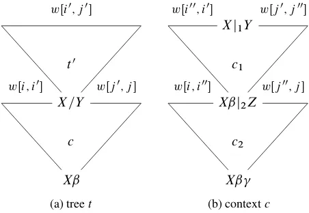
Figure 3: Decomposition of derivations.
4 A Polynomial-Time Algorithm
We now introduce our polynomial-time algorithm. This algorithm uses the same axioms and the same goal item as the CKY-style algorithm, but features new items and new inference rules.
4.1 New Items
In a first step, in order to avoid runtime exponential innwe restrict our item set to categories whose arity is bounded by some grammar constantcG:
ŒX; i; j where ar.X /cG
The exact choice of the constant will be discussed in Section 5. With the restricted item set, the new algorithm behaves like the old one as long as the arity of categories does not exceedcG. However, rule (1)
alone is no longer complete: Derivations with cate-gories whose arity exceedscG cannot be simulated
anymore. To remedy this deficiency, we introduce a new type of item to implement a specific decomposi-tion of long derivadecomposi-tions into smaller pieces.
Consider a derivationt of the form shown in Fig-ure 3(a). Note that the yield oft is wŒi; j . The derivation consists of two parts, namedt0andc; these share a common node with a category of the form X =Y. Now assume thatc has the special property that none of the combinatory rules that it uses pops the argument stack of the categoryX. This means that c, after popping the argument =Y, may push new arguments and pop them again, but may never “touch”X. We call a fragment with this special prop-erty aderivation context. (A formal definition will be given in Section 5.2.)
The special property ofc is useful because it im-plies thatc can be carried out for any choice ofX. To be more specific, let us writeˇfor the (possibly empty) sequence of arguments thatc pushes to the argument stack ofX in place of=Y. We shall refer to =Y as thebridging argumentand to the sequenceˇ as theexcess ofc. Suppose now that we replacet0 by a derivation tree with the same yield but with a typeX0=Y whereX0¤X. Then becausecdoes not touchX0we obtain another valid derivation tree with the same yield ast; the type of this tree will beX0ˇ.
For the combination withc, the internal structure oft0is of no importance; the only important informa-tion is the extent of the yield oft0and the identity of the bridging argument=Y. In terms of our deduction system, this can be expressed as follows: The deriva-tion contextccan be combined with any treet0that is associated with an item of the formŒX =Y; i0; j0, whereX is any category. Similarly, the internal struc-ture ofc is of no importance either, as long as the argument stack of the categoryX remains untouched. It suffices to record the following:
the extent of the yield oft, specified in terms of the positionsi andj;
the extent of the yield oft0, specified in terms of the positionsi0andj0;
the bridging argument=Y; and
the excessˇ.
We represent these pieces of information in a new type of item of the formŒ=Y; ˇ; i; i0; j0; j . The in-tended interpretation of these items is to assert that, for any choice of X, if we can build a derivation treet0 with yieldwŒi0; j0and typeX =Y, then we can also build a derivation treet0with yieldwŒi; j and typeXˇ. We also use items Œ = Y; ˇ; i; i0; j0; j with a backward slash, with a similar meaning. Like items that represent derivation trees, our items for derivation contexts are arity-restricted:
ŒjY; ˇ; i; i0; j0; j where ar.Yˇ/cG
ŒA; 0; 1
ŒS =H = A=F; 2; 5 ŒB; 1; 2
ŒC = A=F; 2; 3
ŒS =E; 3; 4 ŒE=H = C; 4; 5 ŒS =H = C; 3; 5 (1)
ŒS =H = A=F; 2; 5 (1) ŒF =G = B; 5; 6 Œ=F; =G = B; 2; 2; 5; 6 (2)
Œ=F; =G; 1; 2; 5; 6 (4) ŒG; 6; 7
Œ=F; "; 1; 2; 5; 7 (4)
ŒS =H = A; 1; 7 (3)
ŒS =H; 0; 7 (1) ŒH; 7; 8
[image:5.612.83.534.55.168.2]ŒS; 0; 8 (1)
Figure 4: A sample derivation of the grammatical deduction system of Section 4. Inferencetriggers a new context item from a tree item; inferencereuses the tree item (as indicated by the arrow), recombining it with the (modified) context item.
4.2 New Inference Rules
In our parsing algorithm, context items are introduced whenever the composition of two categories whose arities are bounded bycG would result in a category
whose arity exceeds this bound:
ŒX =Y; i; j ŒYˇ; j; k Œ=Y; ˇ; i; i; j; k
8 < :
X =Y Yˇ)Xˇ
ar.Xˇ/ > cG (2)
The new rule has the same antecedents as rule (1), but rather than extending the derivation asserted by the first antecedentŒX =Y; i; j , which is not possible be-cause of the arity bound, it triggers a new derivation context, asserted by the itemŒ=Y; ˇ; i; i; j; k. Fur-ther applications and compositions will extend the new context, and only when the excess of this context has become sufficiently small will it be recombined with the derivation that originally triggered it. This is done by the following rule:
ŒXjY; i0; j0 ŒjY; ˇ; i; i0; j0; j
ŒXˇ; i; j (3)
Note that this rule (like all rules in the deduction system) is only defined on valid items; in particular it only fires if the arity of the categoryXˇis bounded bycG.
The remaining rules of the algorithm parallel the three rules that we have introduced so far but take items that represent derivation contexts rather than derivation trees as their first antecedents. First out, rule (4) extends a derivation context in the same way as rule (1) extends a derivation tree.
ŒjY; ˇ=Z; i; i0; j0; j ŒZ; j; k ŒjY; ˇ; i; i0; j0; k
8 < :
X =Z Z)X
ar.Yˇ /cG
(4)
Rule (5) is the obvious correspondent of rule (2): It triggers a new context when the antecedent context cannot be extended because of the arity bound.
ŒjY; ˇ=Z; i; i0; j0; j ŒZ; j; k Œ=Z; ; i; i; j; k
8 < :
X =Z Z)X
ar.Yˇ / > cG
(5)
Finally, and parallel to rule (3), we need a rule to recombine a context with the context that originally triggered it. As it will turn out, we only need this in cases where the triggered context has no excess.
Œj1Y; ˇj2Z; i00; i0; j0; j00 Œj2Z; "; i; i00; j00; j Œj1Y; ˇ; i; i0; j0; j (6)
4.3 Sample Derivation
We now illustrate our algorithm on a toy grammar. The grammar has the following lexicon:
w1WDA w5WDE=H = C
w2WDB w6WDF =G = B
w3WDC = A=F w7WDG
w4WDS =E w8WDH
The start symbol is S. The grammar allows all in-stances of application and all inin-stances of composi-tion with degree bounded by 2. We letcG D3(as
explained later in Section 5.2).
A derivation of our deduction system on the in-put stringw1 w8 is given in Figure 4. We start
a category with arity 4, exceeding the arity bound. We therefore use rule (2) to trigger the context itemŒ=F; =G = B; 2; 2; 5; 6(). Successively, we use rule (4) twice to obtain the itemŒ=F; "; 1; 2; 5; 7. At this point we use rule (3) (withˇD") to recombine the context item with the tree item that originally triggered it (); this yields the itemŒS =H = A; 1; 7. Note that the recombination effectively retrieves the portion of the stack that was below the argument=F when the context item was triggered in. Double ap-plication of rule (1) produces the goal itemŒS; 0; 8. 4.4 Runtime Analysis
We now turn to an analysis of the runtime complexity of our algorithm. We first consider runtime complex-ity with respect to the length of the input string,n. The runtime is dominated by the number of instantia-tions of rule (6) which involves two context items as antecedents. By inspection of this rule, we see that the number of possible instantiations is bounded by n6. Therefore we conclude that the algorithm runs in timeO.n6/.
We now consider runtime complexity with respect to the size of the input grammar. Here the runtime is dominated by the number of instantiations of rules (1)–(5). For example, rule (5) combines items
ŒjY; ˇ=Z; i; i0; j0; j and ŒZ; j; k : By our restrictions on items, both the arity ofYˇ=Z and the arity ofZ are upper-bounded by the con-stantcG. Now recall that every categoryX can be
written asX DA˛for some atomic categoryAand stack of arguments˛. LetA be the set of atomic categories in the input grammar, and let L be the set of all arguments occurring in any category of the lexicon. By a result of Vijay-Shanker and Weir (1994, Lemma 3.1), every argument that may occur in a derived category occurs inL. Then the number of possible instantiations of rule (5) as well as rules (1)–(4), and hence the runtime of the algorithm, is in
O.jAj jLjcG
jLjcG/
DO.jAj jLj2cG/ :
Note that bothAandLmay grow with the grammar size. As we will see in Section 5.2, the constantcG
also depends on the grammar size. This means that the worst-case runtime complexity of our parser is exponential in the size of the input grammar. We will return to this point in Section 7.
5 Correctness
In this section we prove the correctness of our parsing algorithm. In order to simplify the proofs, we start by simplifying our algorithm, at the cost of making it less efficient:
We remove the rules for extending trees and
contexts, rule (1) and rule (4).
We conflate the rules for triggering contexts,
rule (2) and rule (5), into the single rule ŒYˇ; j; k
Œ=Y; ˇ; i; i; j; k X =Y Yˇ)Xˇ (7) This rule blindly guesses the extension of the triggering tree or context (specified by posi-tions i and j), rather than waiting for a cor-responding item to be derived.
The simplified algorithm is specified in Figure 5. We now argue that this algorithm and the algorithm from Section 4 parse exactly the same derivation trees, although they use different parsing strategies. First, we observe that rule (1) in the old algorithm can be simulated by a combination of other rules in the simplified algorithm, as follows:
ŒX =Y; i; j
ŒYˇ; j; k Œ=Y; ˇ; i; i; j; k (7)
ŒXˇ; i; k (3)
Furthermore, the simplified algorithm does no longer need rule (4), whose role is now taken over by rule (7). To see this, recall that rule (4) extends an existing context whenever the composition of two categories results in a new category whose arity does not exceedcG. In contrast, rule (7)alwaystriggers a
new contextc, even if the result of the composition ofc with some existing context satisfies the above arity restriction. Despite the difference in the adopted strategy, these two rules are equivalent in terms of stack content, leading to the same derivation trees. 5.1 Definitions
We introduce some additional terminology and nota-tion that we will use in the proofs. For a derivanota-tion treet and a nodeuoft, we writet Œuto denote the category atu, and we writetju to denote the
sub-tree oft atu. Formally,tjuis the restriction oft to
Items of type 1: ŒX; i; j , ar.X /cG Items of type 2: ŒjY; ˇ; i; i0; j0; j , ar.Yˇ/cG
Axioms: ŒX; i; iC1, wiC1WDX Goal: ŒS; 0; n
Inference rules: ŒYˇ; j; k
Œ=Y; ˇ; i; i; j; k X =Y Yˇ)Xˇ (7)
ŒX =Y; i0; j0 Œ=Y; ˇ; i; i0; j0; j ŒXˇ; i; j (3)
Œj1Y; ˇj2Z; i00; i0; j0; j00 Œj2Z; "; i; i00; j00; j
Œj1Y; ˇ; i; i0; j0; j
[image:7.612.126.497.72.161.2](6)
Figure 5: Items and inference rules of the simplified algorithm for an input stringw1 wn.
Definition 1 Lett be a derivation tree with rootr. Thent hassignatureŒX; i; j if
1. the yield oft iswŒi; j and
2. the type oftisX, that is,t ŒrDX.
Note that while we use the same notation for sig-natures as for items, the signature of a derivation tree is a purely structural concept, whereas an item is an object in the algorithm.
A central concept in our proof is the notion of
spine. Recall that a derivation tree consists of unary branchings and binary branchings. In each binary branching, we refer to the two children of the branch-ing’s root node as the primary child and the sec-ondary child, depending on which of the two is la-beled with the primary and secondary input category of the corresponding rule instance. In Figure 2, the primary children of the root node are shaded. Definition 2 For a derivation treet, thespineoftis the unique path that starts at the root node oftand at each nodeucontinues to the primary child ofu.
The spine of a derivation tree always ends at a node that is labeled with a category from the lexicon. Definition 3 Lett be a derivation tree with rootr. Aderivation contextc is obtained by removing all proper descendants of some nodef ¤ron the spine oft, under the restriction thatar.t Œu/ >ar.t Œr/for every nodeuon the spine properly betweenf andr. The nodef is called thefoot nodeofc. Theyield ofc is the pair whose first component is the yield oft to the left off and whose second component is the yield oft to the right off. For a derivation contextcand a nodeuofc, we writecŒuto denote the category atu.
Definition 3 formalizes the concept of derivation contexts that we introduced in Section 4.1. First, because f is on the spine and f ¤ r, the cate-gorycŒf takes the form X =Y. The arity restric-tion implies that the category of every nodeuon the spine properly betweenf andrtakes the formXˇu,
jˇuj> 0, and that the category at the root takes the
form Xˇ, jˇj 0. Thus the category X is never exposed inc, except perhaps at r. As we will see in Section 5.4, this property, together with a careful selection of “split nodes”, will allow us to decompose derivations into smaller, shareable parts. The basic idea is the same as in the tabulation of pushdown automata (Lang, 1974; Nederhof and Satta, 2004), where the pushdown in our case is the argument stack of the primary input categories along a spine.
The concepts of signature and spine are general-ized to derivation contexts as follows:
Definition 4 Letcbe a derivation context with root node r and foot node f. Then c has signature ŒjY; ˇ; i; i0; j0; j if
1. the yield ofc is.wŒi; i0; wŒj0; j /; 2. for someX,cŒf DXjY andcŒrDXˇ. Definition 5 For a derivation contextc, the spine ofcis the path from its root node to its foot node. 5.2 Grammar Constant
Before we start with the proof as such, we turn to the choice of the grammar constantcG, which was
left pending in previous sections. Recall that we are usingcG as a bound on the arity ofX in type 1
itemsŒX; i; j . Since these items are produced by our axioms from the set of categories in the lexicon, cG must not be smaller than the maximum arity`of
We also usecG as a bound on the arity of the
cat-egoryYˇ in type 2 itemsŒjY; ˇ; i; i0; j0; j . These items are produced by inference rule (7) to simulate instances of composition of the formX =Y Yˇ ) Xˇ. Here the length of ˇis bounded by the maxi-mum degreed of a composition rule in the grammar, andar.Y /is bounded by the maximum arityaof an argument from the (finite) setLof arguments in the lexicon (recall Section 4.4). ThereforecG cannot be
smaller thanaCd. Putting everything together, we obtain the condition
cG maxf`; aCdg: (8)
The next lemma will be used in several places later. Lemma 1 Letcbe a derivation context with
signa-tureŒjY; ˇ; i; i0; j0; j . Then ar.Yˇ/cG.
Proof. Let r and f be the root and the foot node, respectively, ofc. From the definition of signature, there must be some X such that cŒr D Xˇ and cŒf D XjY. Now letp be the parent node off, and assume that the rule used atpis instantiated as X =Y Yˇ0 ) Xˇ0, so thatcŒp D Xˇ0. Ifp D r thenˇ0Dˇ; otherwise, because of the arity restric-tion in the definirestric-tion of derivarestric-tion contexts (Defini-tion 3) we havejˇ0j>jˇj. Then
ar.Yˇ/ar.Yˇ0/cG;
where the right inequality follows from the assump-tion thatX =Y Yˇ0)Xˇ0is a rule instance of the grammar, and from inequality (8).
5.3 Soundness
We start the correctness proof by arguing for the soundness of the deduction system in Figure 5. More specifically, we show that for every item of type 1 there exists a derivation tree with the same signa-ture, and that for every item of type 2 there exists a derivation context with the same signature.
The soundness of the axioms is obvious.
Rule (7) states that, if we have built a derivation treet with signatureŒYˇ; j; kthen we can build a derivation contextcwith signatureŒ=Y; ˇ; i; i; j; k. Under the condition that the grammar admits the rule instanceX =Y Yˇ ) Xˇ, this inference is sound; the context can be built as shown in Figure 6.
wŒj; k
Yˇ X =Y
[image:8.612.382.474.56.122.2]Xˇ t
Figure 6: Soundness of rule (7).
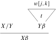
Rule (3) states that, if we have built a derivation treet0with signature ŒX =Y; i0; j0and a context c with signatureŒ=Y; ˇ; i; i0; j0; j , then we can build a new treetwith signatureŒXˇ; i; j . We obtaint by substitutingt0for the foot node ofc(see Figure 3(a)). Rule (6) states that, if we have built a derivation contextc1 with signature Œj1Y; ˇj2Z; i00; i0; j0; j00
and another context c2 with signature
Œj2Z; "; i; i00; j00; j , then we can build a derivation
context c with signature Œj1Y; ˇ; i; i0; j0; j . We
obtainc by substitutingc1 for the foot node ofc2;
this is illustrated by Figure 3(b) if we assume D".
5.4 Completeness
In the final part of our correctness proof we now prove the completeness of the deduction system in Figure 5. Specifically we show the following stronger statement: For every derivation tree and for every derivation context with a signatureI satisfying the arity bounds for items of Figure 5, the deduction system infers the corresponding itemI. From this statement we can immediately conclude that the sys-tem constructs the goal isys-tem whenever there exists a derivation tree whose yield is the complete input string and whose type is the distinguished categoryS.
Our proof is by induction on a measure that we callrank. The rank of a derivation tree or context is the number of its non-leaf nodes. Note that this definition implies that the foot node of a context is not counted against its rank. The rank of a tree or context is always at least 1, with rank1only realized for derivation trees consisting of a single node.
5.4.1 Base Case
Consider a derivation treetwith signatureŒX; i; j andrank.t / D1. The treet takes the form shown in the left of Figure 2, and we havej Di C1and wj WDX. The itemŒX; i; j is then produced by one
5.4.2 Inductive Case
The general idea underlying the inductive case can be stated as follows. We consider a derivation tree or context'with signatureI satisfying the bounds stated in Figure 5 for items of type 1 or 2. We then identify a special nodesin'’s spine, which we call thesplitnode. We usesto “split”' into two parts that are either derivation trees or contexts, that both satisfy the bounds for items of type 1 or 2, and that both have rank smaller than the rank of'. We then apply the induction hypothesis to obtain two items that can be combined by one of the inference rules of our algorithm, resulting in the desired itemI for'. We first consider the case in which' is a tree, and later the case in which' is a context.
5.4.3 Splitting Trees
Consider a derivation tree t with signature ŒX0; i; j , root node r, andrank.t / > 1. Then the spine oft consists of at least 2 nodes. Now assume thatar.X0/cG, that is,ŒX0; i; j is a valid item.
Choose the split nodesto be the highest (closest to the root) non-root node on the spine for which
ar.t Œs/ cG. Node s always exists, as the arity
constraint is satisfied at least for the lowest (farthest from the root) node on the spine, which is labeled with a category from the lexicon.
Consider the subtreet0 D tjs; thuss is the root
node of t0. Because s is a primary node in t, the category at s has at least one argument. We deal here with the case where this category takes the form t Œs D X =Y; the case t Œs D X = Y is sym-metrical. Thus the signature of t0 takes the form ŒX =Y; i0; j0wherei0; j0are integers withi i0< j0 j. By our choice of s, ar.X =Y / cG, and
thereforeŒX =Y; i0; j0is a valid item. Furthermore,
rank.tjs/ <rank.t /, asrdoes not belong totjs. We
may then use the induction hypothesis to deduce that our algorithm constructs the itemŒX =Y; i0; j0.
Now consider the contextcthat is obtained fromt by removing all proper descendants ofs; thusris the root node ofcandsis its foot node. To see thatcis well-defined, note that our choice ofsguarantees that
ar.t Œu/ >ar.t Œr/for every nodeuthat is properly betweens and r: If there was a node usuch that
ar.t Œu/ ar.t Œr/then because oft Œr D X0and our assumption thatar.X0/ cG we would have
chosenuinstead ofs.
Now letˇ be the excess ofc; thenX0 Dt ŒrD t ŒsˇDXˇ. Thus the signature ofctakes the form Œ=Y; ˇ; i; i0; j0; j . Applying Lemma 1 toc, we get
ar.Yˇ/ cG, and therefore Œ=Y; ˇ; i; i0; j0; j is
also a valid item. Furthermore,rank.c/ <rank.t /, since nodesis counted inrank.t /but not inrank.c/. By the induction hypothesis, we conclude that our algorithm constructs the itemŒ=Y; ˛; i; i0; j0; j .
Finally, we apply the inference rule (3) to the previously constructed items ŒX =Y; i0; j0 and Œ=Y; ˇ; i; i0; j0; j . This yields the itemŒXˇ; i; j D
ŒX0; i; j fort, as desired. 5.4.4 Splitting Contexts
Consider a derivation context c with signature Œ=Y; ˇ; i; i0; j0; j , root r, and foot f. (The case where we have = Y instead of =Y can be covered with a symmetrical argument.) From Definition 4 we know that there is a categoryX such thatcŒf D X =Y and cŒr D Xˇ, and from the definition of context we know that for every spinal nodeuthat is properly betweenf andr it holds thatar.cŒu/ >
ar.cŒr/. Now assume that ar.Yˇ/ cG, that is,
Œ=Y; ˇ; i; i0; j0; j is a valid item. We distinguish two cases below.
Case 1 Suppose that the spine ofc consists of ex-actly 2 nodes. In this case the footf is the left child of the rootrandi Di0. Letf0be the right sibling off and consider the subtree t0 D tjf0; thus f0
is the root node oft0. The signature oft0takes the formŒYˇ; j0; j . By our assumption,ar.Yˇ/cG,
and then ŒYˇ; j0; j is a valid item. Furthermore,
rank.t0/ <rank.c/since the root noderis counted inrank.c/but not inrank.t0/. Then, by the induction hypothesis, the itemŒYˇ; j0; j is constructed by our algorithm. We now apply inference rule (7) to this item; this yields the itemŒ=Y; ˇ; i; i0; j0; j forc, as required.
Case 2 Suppose that the spine ofcconsists of more than 2 nodes. This means that there is at least one spinal node that is properly betweenf andr.
nodeuin the spine, and at the same time, no combi-natory rule can reduce the arity of its primary input category by more than one unit.
Consider the contextc1that is obtained by
restrict-ing c to node s and all of its descendants; thus s is the root node of c1 and f is the foot node. To
see thatc1is well-defined, note that our choice ofs
guarantees thatar.cŒu/ > ar.cŒs/for every node u that is properly between f and s. To see this, suppose that there was a node u ¤ s such that
ar.cŒu/ ar.cŒs/. Sincear.cŒs/ Dar.cŒr/C1 andar.cŒu/¤ ar.cŒs/, by our definition ofs, we would have ar.cŒu/ ar.cŒr/, which cannot be because inc, every nodeuproperly betweenf and shas arityar.cŒu/ >ar.cŒr/.
Becausef is a primary node inc, the category at f has at least one argument; call itj1Y. The node
s is a primary node inc as well, so the excess of c1 takes the formˇj2Z, wherej2Z is the topmost
argument of the category at s. Thus the signature ofc1takes the formŒj1Y; ˇj2Z; i00; i0; j0; j00where
i00; j00are integers withi i00 i0andj0j00 j. Applying Lemma 1 toc1, we getar.Yˇj2Z/
cG, and thereforeŒj1Y; ˇj2Z; i00; i0; j0; j00is a valid
item. Finally, we note thatrank.c1/ <rank.c/, since
the root noder is counted inc but not inc1. By the
induction hypothesis we conclude that our algorithm constructs the itemŒj1Y; ˇj2Z; i00; i0; j0; j00.
Now consider the contextc2that is obtained from
cby removing all proper descendants of the nodes; thusr is the root node ofc2andsis the foot node.
To see thatc2 is well-defined, note thatar.cŒu/ > ar.cŒr/for every nodeuthat is properly betweens andrsimply because every such node is also properly betweenf and r. The excess of c2 is the empty
stack " by our choice ofs. Thus the signature of c2isŒj2Z; "; i; i00; j00; j . We apply Lemma 1 once
more, this time toc2, to show thatar.Z/cG, and
conclude thatŒj2Z; "; i; i00; j00; j is also a valid item.
Finally we note thatrank.c2/ <rank.c/, as the node
s is counted in c but not in c2. By the induction
hypothesis we conclude that our algorithm constructs the itemŒj2Z; "; i; i00; j00; j .
We now apply inference rule (6) to the pre-viously constructed items Œj1Y; ˇj2Z; i00; i0; j0; j00
and Œj2Z; "; i; i00; j00; j . This yields the item
Œj1Y; ˇ; i; i0; j0; j as desired.
6 Discussion
We round off the article with a discussion of our algorithm and possible extensions.
6.1 Support for Rule Restrictions
As we mentioned in Section 2, the CCG formalism of Weir and Joshi (1988) allows a grammar to impose certain restrictions on valid rule instances. More specifically, for every rule a grammar may restrict (a) the target of the primary input category and/or (b) parts of or the entire secondary input category.3
The algorithm in Figure 5 can be extended to sup-port such rule restrictions. Note that already in its present form, the algorithm only allows inferences that are licensed by valid instances of a given rule. Supporting restrictions on the secondary input cat-egory (restrictions of type b) is straightforward— assuming that these restrictions can be efficiently tested. To also support restrictions on the target of the primary input category (restrictions of type a) the items can be extended by an additional component that keeps track of that target category for the cor-responding derivation subtree or context. With this information, rule (7) can perform a check against the restrictions specified for the composition rule, and rules (3) and (6) merely need to test whether the tar-get categories of their two antecedents match, and propagate the common target category to the conclu-sion. This is essentially the same solution as the one adopted in the V&W algorithm.
6.2 Support for Multi-Modal CCG
The modern version of CCG has abandoned rule restrictions in favor of a new, lexicalized control mechanism in the form ofmodalitiesorslash types
(Steedman and Baldridge, 2011). However, as shown by Baldridge and Kruijff (2003), every multi-modal CCG can be translated into an equivalent CCG with rule restrictions. The basic idea is to specialize the target of each category and argument for a slash type, and to reformulate the multi-modal rules as rules with restrictions that reference this information. With this simulation, our parsing algorithm can also be used as a parsing algorithm for multi-modal CCG.
3Such restrictions can be used, for example, to impose the
linguistically relevant distinction betweenharmonicandcrossed
6.3 Comparison with the V&W Algorithm As already mentioned in Section 1, apart from the algorithm presented in this article, the only other algorithm known to run in polynomial time in the length of the input string is the one presented by Vijay-Shanker and Weir (1993). At an abstract level, the two algorithms are based on the same basic idea of decomposing CCG derivations into pieces of two different types, one of which spans a portion of the input string that includes a gap. This idea actually underlies several parsing algorithms for equivalent mildly context-sensitive formalisms, such as Tree-Adjoining Grammar (Joshi and Schabes, 1997).
The main difference between the V&W algorithm and the one presented in this article is the use of different decompositions for CCG derivations. In our algorithm we allow the excess of a derivation context to be the empty list of arguments, something that is not possible in the V&W algorithm. There, when an application operation empties the excess ˇof some context, one is forced to retrieve, in the same elementary step, the portion of the stack placed right belowˇ. This requires the distinction of several possible cases, resulting in four different realizations of the application rule (Vijay-Shanker and Weir, 1993, p. 616). As a consequence, the V&W algorithm uses nine (forward) inference rules, against our algorithm in Figure 5 which uses only three. Furthermore, some of the inference rules in the V&W algorithm use three antecedent items, while our use a maximum of two. This results in a runtime complexity of O.n7/ for the V&W algorithm,nthe length of the input string; however, Vijay-Shanker and Weir (1993) show how their algorithm can be implemented in timeO.n6/at the cost of some extra bookkeeping. In contrast, our algorithm directly runs in timeO.n6/.
The relative proliferation of inference rules, com-bined with the increase in their complexity, makes, in our own opinion, the specification of the V&W parser more difficult to understand and implement, and calls for a more articulated correctness proof.
6.4 Support for Additional Types of Rules Like the V&W algorithm, our algorithm currently only supports (generalized) composition but no other combinatory rules required for linguistic analysis, in particular type-raising and substitution.
Type-raising is a unary rule of the (forward) form X ) T =.T = X / whereT is a variable over cate-gories. Under the standard assumption thatT = X is limited to a finite set of categories (Steedman, 2000), this rule can be implemented in our algorithm by introducing a new unary inference rule and choos-ing the constantcGlarge enough to accomodate all
instances ofT = X.
Substitution is a binary rule of the (forward) form X =YjZ YjZ ) X =Z. This rule is easy to imple-ment if both=Y andjZare stored in the same item. Otherwise, we need to passjZ to any item storing the=Y. This can be done by changing the second antecedent of rule (6) to allow a single argument
jZinstead of the empty excess". The price of this change is spurious ambiguity in the derivations of the grammatical deduction system.
7 Conclusion
Recently, there has been a surge of interest in the mathematical properties of CCG; see for in-stance Hockenmaier and Young (2008), Koller and Kuhlmann (2009), Fowler and Penn (2010) and Kuhlmann et al. (2010). Following this line, this article has revisited the parsing problem for CCG.
Our work, like the polynomial-time parsing algo-rithm previously discovered by Vijay-Shanker and Weir (1993), is based on the idea of decomposing large CCG derivations into smaller, shareable pieces. Here we have proposed a derivation decomposition different from the one adopted by Vijay-Shanker and Weir (1993). This results in an algorithm which, in our own opinion, is simpler and easier to understand.
Although we have specified only a recognition version of the algorithm, standard techniques can be applied to obtain a derivation forest from our parsing table. This consists in saving backpointers at each inference rule, linking newly inferred items to their antecedent items.
Acknowledgments
We thank the Action Editor and the reviewers for their detailed and insightful feedback on the first version of this article. GS has been partially supported by MIUR under project PRIN No. 2010LYA9RH_006.
References
Jason Baldridge and Geert-Jan M. Kruijff. 2003. Multi-modal combinatory categorial grammar. InTenth Con-ference of the European Chapter of the Association
for Computational Linguistics (EACL), pages 211–218,
Budapest, Hungary.
Johan Bos, Stephen Clark, Mark Steedman, James R. Cur-ran, and Julia Hockenmaier. 2004. Wide-coverage semantic representations from a CCG parser. In Pro-ceedings of the 20th International Conference on
Com-putational Linguistics (COLING), pages 1240–1246,
Geneva, Switzerland.
Stephen Clark and James R. Curran. 2007. Wide-coverage efficient statistical parsing with CCG and log-linear models.Computational Linguistics, 33(4):493– 552.
Timothy Fowler and Gerald Penn. 2010. Accurate context-free parsing with combinatory categorial gram-mar. InProceedings of the 48th Annual Meeting of
the Association for Computational Linguistics (ACL),
pages 335–344, Uppsala, Sweden.
Julia Hockenmaier and Peter Young. 2008. Non-local scrambling: The equivalence of TAG and CCG revis-ited. In Ninth International Workshop on Tree
Ad-joining Grammars and Related Formalisms (TAG+),
Tübingen, Germany.
Aravind K. Joshi and Yves Schabes. 1997. Tree-Adjoining Grammars. In Grzegorz Rozenberg and Arto Salomaa, editors,Handbook of Formal Languages, vol-ume 3, pages 69–123. Springer.
Aravind K. Joshi. 1985. Tree Adjoining Grammars: How much context-sensitivity is required to provide reason-able structural descriptions? In David R. Dowty, Lauri Karttunen, and Arnold M. Zwicky, editors,Natural
Lan-guage Parsing, pages 206–250. Cambridge University
Press.
Alexander Koller and Marco Kuhlmann. 2009. Depen-dency trees and the strong generative capacity of CCG.
InProceedings of the 12th Conference of the European
Chapter of the Association for Computational
Linguis-tics (EACL), pages 460–468, Athens, Greece.
Marco Kuhlmann, Alexander Koller, and Giorgio Satta. 2010. The importance of rule restrictions in CCG. In
Proceedings of the 48th Annual Meeting of the
Asso-ciation for Computational Linguistics (ACL), pages
534–543, Uppsala, Sweden.
Tom Kwiatkowski, Luke Zettlemoyer, Sharon Goldwater, and Mark Steedman. 2010. Inducing probabilistic CCG grammars from logical form with higher-order unification. InProceedings of the 2010 Conference on Empirical Methods in Natural Language Processing
(EMNLP), pages 1223–1233, Cambridge, MA, USA.
Bernard Lang. 1974. Deterministic techniques for ef-ficient non-deterministic parsers. In Jacques Loecx, editor,Automata, Languages and Programming, 2nd Colloquium, University of Saarbrücken, July 29–August
2, 1974, number 14 in Lecture Notes in Computer
Sci-ence, pages 255–269. Springer.
Mike Lewis and Mark Steedman. 2013. Combined distri-butional and logical semantics.Transactions of the
As-sociation for Computational Linguistics, 1(May):179–
192.
Mark-Jan Nederhof and Giorgio Satta. 2004. Tabular parsing. In Carlos Martín-Vide, Victor Mitrana, and Gheorghe P˘aun, editors,Formal Languages and
Appli-cations, volume 148 ofStudies in Fuzziness and Soft
Computing, pages 529–549. Springer.
Remo Pareschi and Mark Steedman. 1987. A lazy way to chart-parse with categorial grammars. InProceedings of the 25th Annual Meeting of the Association for
Com-putational Linguistics (ACL), pages 81–88, Stanford,
CA, USA.
Stuart M. Shieber, Yves Schabes, and Fernando Pereira. 1995. Principles and implementation of deductive
pars-ing.Journal of Logic Programming, 24(1–2):3–36.
Mark Steedman and Jason Baldridge. 2011. Combinatory categorial grammar. In Robert D. Borsley and Kersti Börjars, editors,Non-Transformational Syntax: Formal
and Explicit Models of Grammar, chapter 5, pages 181–
224. Blackwell.
Mark Steedman. 2000. The Syntactic Process. MIT Press.
Masaru Tomita. 1988. Graph-structured stack and natural language parsing. InProceedings of the 26th Annual Meeting of the Association for Computational
Linguis-tics (ACL), pages 249–257, Buffalo, USA.
K. Vijay-Shanker and David J. Weir. 1990. Polynomial time parsing of combinatory categorial grammars. In
Proceedings of the 28th Annual Meeting of the
Associa-tion for ComputaAssocia-tional Linguistics (ACL), pages 1–8,
Pittsburgh, USA.
K. Vijay-Shanker and David J. Weir. 1993. Parsing some constrained grammar formalisms. Computational
Lin-guistics, 19(4):591–636.
K. Vijay-Shanker and David J. Weir. 1994. The equiv-alence of four extensions of context-free grammars.
Mathematical Systems Theory, 27(6):511–546.
rules. InProceedings of the Seventh Workshop on
Sta-tistical Machine Translation, pages 222–231, Montréal,
Canada.
David J. Weir and Aravind K. Joshi. 1988. Combinatory categorial grammars: Generative power and relation-ship to linear context-free rewriting systems. In Pro-ceedings of the 26th Annual Meeting of the Association
for Computational Linguistics (ACL), pages 278–285,