Modelling and Planning the Migration for Next Generation Networks

(1)

Modelling and Planning the Migration for Next

Generation Networks

by

Mathieu Robin

A thesis submitted to

the University of Dublin

for the degree of

Master of Science in Computer Science

(2)

Declaration

This thesis has not been submitted as an exercise for a degree at any other University. Except where otherwise stated, the work described herein has been carried out by the author alone. This thesis may be borrowed or copied upon request with the permission of the Librarian, University of Dublin, Trinity College. The copyright belongs jointly to the University of Dublin and Mathieu Robin.

(3)

Acknowledgements

I would like to thank my supervisor, Meriel Huggard, for her enthusiasm and

guidance throughout the course of this project. I would also like to thank the people

at Eircom involved in this project, David Blair and Lorcan Dillon-Kelly. Finally I

would like to thank my friends and classmates for their continuous support throughout

(4)

Abstract

The ever increasing volume of data traffic on telecommunications networks has led

to a fundamental shift in network operator requirements. Moreover, the continuous

evolution of the industry, with developments such as mobile telephony, has created a

need for interoperability and advanced service management.

These changes in network usage have given rise to major infrastructural change:

telecommunication networks are moving from switched circuit networks, designed

to handle telephony service, to multi-service digital technologies. This evolution is

referred as the migration to Next Generation Networks.

The development of a computer-based tool for modelling and planning this migration

is outlined. This may be used to study the main characteristics of the new network

infrastructure. The tool focuses on network dimensioning and quality of service:

Algorithms have been created to study how migration affects capacity requirements

(5)

List of Tables

2.1 Intserv/ATM Service Class mapping . . . 12

5.1 Traffic Types . . . 38

7.1 Traffic matrix . . . 59

(10)

List of Figures

3.1 Network simulation models . . . 20

4.1 Class Diagram . . . 31

4.2 Example Network . . . 32

5.1 Traffic types . . . 38

6.1 Example Network . . . 44

6.2 Events Relationships . . . 45

6.3 Example Source Bit Rate . . . 47

6.4 Example: Constant Bit Rate . . . 48

6.5 Markov-Modulated Rate Process . . . 48

6.6 Example: Markov-Modulated Process . . . 49

6.7 Markov-Modulated On-Off . . . 49

6.8 Example: On-Off Sources . . . 50

6.9 Sample flow evolution . . . 54

7.1 Eircom Network . . . 58

7.2 Test Network . . . 61

7.3 Test Sources Output . . . 62

7.4 Delay / Service Rate . . . 63

7.5 Loss / Service Rate . . . 63

7.6 Buffer size influence . . . 65

(11)

7.8 Loss Ratio Study . . . 66

7.9 Loss Ratio Study - A/B . . . 67

(12)

Chapter 1 Introduction

This thesis describes the work carried out to design and implement an improved

version of a computer-based tool to model the migration to Next Generation Networks

(NGN).

Telecommunication network operators use the term migration to Next Generation

Networks to refer to the process of moving from a network infrastructure designed to

handle voice communication to a multi-service digital one.

1.1 Context

The use of the telecommunication networks to carry data and real-time services

has changed the requirements in terms of infrastructure and technology. Currently,

services tend to be provided on dedicated networks. It is envisaged that these will be

replaced by NGNs which provide integrated multi-service networks.

Today, the telecom operators are engaged in modifications and updates of their

trans-port network. Even if the technologies involved are well established, for example IP

and ATM, the path of migration is still unclear.

This migration has started in the mid 1990s, but most operators still have to make

(13)

infrastructure. As stated in [Don01], the motivations behind the migration are:

• The high growth of the Internet, which implies an increase of a world wide IP

traffic,

• The growth of mobile telephony, and the change to a multi-operator competitive

environment,

• The increasing complexity of network and service management.

However, a lot of issues arise regarding the deployment of the NGNs:

• Cost: The migration has to be cost effective, bearing in mind that the revenue

brought in by classic telephony is decreasing.

• Quality of Service: The customers expect perfect quality of service (QoS) for voice traffic, and such QoS is not easily achievable on cell/packet switching

networks.

• Planning: Forecasting of demand and network planning are harder for data traffic; the models involved are more complex than the ones used for telephony.

• Underlying technology: For packet-based, multi-service networks, two technolo-gies exist: IP and ATM. However, it is difficult to choose between these; both

are supported by different players of the telecommunications community.

The use of planning tools to assist telecommunication operators in their investments

through the migration steps is needed.

We will detail NGNs and the migration to these networks in chapter 2.

1.2 Project Goal

The project statement is to provide easy and fast ways to forecast the advantages

(14)

As this work is based on a project funded by Eircom ([Hov01]), the collaboration

with this telecom operator has been used: Eircom has provided information

regard-ing traffic model, a realistic network infrastructure, and some general consideration

regarding the migration to NGNs.

1.2.1 Previous Work

The main goal of this project is the validation and the improvement of a

computer-based tool developed by Eirik Hovland in 2001 ([Hov01]).

This tool has two main features:

• Traffic growth planning: Using the Kruithoff algorithm, the tool is able to esti-mate traffic needs for the next three years.

• Bandwidth requirement estimation: Given the amount of data transfered during one peak hour, the tool computes an approximation of the bandwidth required

to carry such data efficiently. The source model is taken from the ATM

speci-fication, and sources are supposed to some ATM traffic class. The underlying

network can be PSTN (Public Switched Telephone Network) or ATM.

The most useful feature of this tool has been the bandwidth estimation function.

It allows an easy comparison between the PSTN network and the ATM network,

by estimating the bandwidth gained using ATM instead of PSTN-based networks.

Various network scenarios and traffic mixes may be studied using the planning tool.

1.2.2 Validation of Previous Work

The traffic growth planning feature has not been implemented in the new version,

given the difficulty of traffic growth forecasting in NGNs. Efforts have been focused

on improving the second feature, and adding valuable ones to the tool.

During this first phase, efforts have been focused on improving the scalability and the

(15)

1.2.3 Improvement: Network Simulation

After a first step, during which the algorithms used in Hovland’s project has been

implemented and validated, it has been decided to improve the tool by building a

small network simulator on top of the existing network model, to allow dynamic

stud-ies and not only static bandwidth requirements. The network simulator brings data

such as the delay or the loss ratio in the evaluation of a system.

1.3 Thesis Outline

The next two chapters describe the background research which has been used to

design the second step of the project. Detailed information about the Next

Genera-tion Networks and the current use in the industry are in chapter 2.

The study of network simulation and the implementation of a simple network

sim-ulator represent a significant part of this project. Chapter 3 is a study of the main

algorithms used in network simulation, issues which are rising then writing a network

simulator, and a short review of the simulators currently available on the market.

The general design of the two versions of the planning tool is described in chapter 4.

Details about the implementation of [Hov01] is given in chapter 5, a review of the key

algorithms of the actual implementation of the network simulator is given in chapter

6. Various tests have been carried out, the method used and the results can be found

in chapter 7.

Finally, chapter 8 concludes this thesis, with a detailed analysis of the work carried

(16)

Chapter 2 Migration to Next Generation

Networks

2.1 The Next Generation Networks

For the last 15 years, the telecommunication world has to face new challenges.

The infrastructure and technologies designed to carry only telephony services need

to evolve to cope with the expanding of multimedia and data services. According

to [Don01], “the most striking changes have been in the growth of both the Internet

and mobile telephony”. The new multi-services network has to be build on top of

the legacy equipment of the PSTN, and it is essential that this transition is both

smooth and cost effective. This transformation is referred as the migration to Next

Generation Networks, or NGN. In simple terms this can be described as a transition

from circuit switching to cell switching or packet forwarding.

As stated in [Eri01b] and many other papers, the two technologies of choice for NGNs

are ATM and IP. This chapter will focus on the main advantages and drawbacks of

these technologies.

The main challenge is to provide the customer with the same features he had on PSTN

networks: as a total switched connection protocol it provides a perfect connection

(17)

about the rise of broadband multi-service networks ([Eri01a]). Bennett ([Ben01])

out-lines the importance of reliability on voice over packet connections. Another challenge

facing network operators is to adapt the billing strategies for these technologies. Most

of the following considerations about ATM and IP have been gathered from various

sources, especially [Dan02] and [PD00].

2.2 IP - Internet Protocol

The main characteristics of IP are that it is:

• the underlying technology of the Internet and of almost every LANs,

• highly flexible, and easy to manage,

• designed to scale well and to be fault tolerant,

• the technology of choice for future multimedia services,

• able to provide QoS and traffic engineering (although these are recent additions

to the protocol and are not yet widely applied).

2.2.1 IP Telephony

One of the major fact in favour of the use of IP for NGNs is the growing use of

this technology to carry telephone traffic.

The main benefits of IP telephony are that:

• Customers can take advantage of flat Internet rating to save money on long

distance calls. While classical telephony rates depends of distance and can be

significantly high, the cost of an Internet connection is constant. However, the

prices for both technologies are likely to converge as IP telephony gains market

(18)

• The telephony service could be integrated within the computer environment, al-lowing for the management of phone calls and phone books from sources such as

customer relationship management, sales force automation, supply chain

man-agement, time accounting, etc. (Source: [Gro01]). The integration and

exten-sion of software solutions should reduce the investment in terms of time and

money.

In this section, a short overview of the two main protocols of Voice over IP is

given. These protocols are H.323 and SIP (Session Initiative Protocol).

H.323

H.323 is an ITU-T (International Telecommunication Union) specification for

mul-timedia conferencing over IP. It was designed to address a concern for the requirements

of multimedia communication over IP networks, including audio, video, and data

con-ferencing. The data is encoded in a compact binary format that is suitable for both

narrowband and broadband connections.

H.323 is designed as an unified system, which allows interoperability with legacy

tele-phony systems, along with a level of robustness and reliability that is comparable to

the one of current PSTN technology. Actually, H.323 includes many other standards,

for signalling, real-time voice transports, codecs. It is a peer-to-peer protocol, while

other protocols, such as MGCP1_{, imply a central control.}

SIP

SIP is an IETF (Internet Engineering Task Force) standard for peer-to-peer

multi-media sessions and IP telephony. It is designed to setup a session between two points,

using the Internet architecture. The guarantees of QoS and connectivity are quite

low; SIP has no support for multimedia conferencing and interoperability is not well

supported.

1_{The Media Gateway Control Protocol was designed to simplify the design and cost of IP}

(19)

SIP messages are encoded in ASCII text format: the messages are large and less

suitable for networks where bandwidth, delay, and/or processing are of concern.

Comparison

H.323 is an adaption of existing technology to the Internet, and designed to inter

operate well with the Plain Old Telephony System (POTS). On the other hand, SIP

has less features of the old telephony service, but has been designed to be integrated

among the other Internet applications, allowing telephony from the computer desktop.

As IP does not provide control over intermediate routers involved in a connection, the

only way to ensure good QoS is the use of dynamic routing ([Net99]). Both of the

technologies discussed use dynamic routing. Another common feature is that these

technologies are peer-to-peer.

The differences between the two protocols are due to their respective promoters:

• H.323 has been designed by ITU-T, is promoted by the telecom industry, and

deals with integration with the telecommunication infrastructure;

• SIP is an IETF standard, and thus can be seen as an Internet-based application.

2.3 ATM - Asynchronous Transfer Mode

ATM is a connection-oriented technology, based on packet switching. It rose to

prominence in the 1980s and in the early 1990s, because it was the technology of

choice of telecom industry, and at this time had a lot of interesting features for LAN

networking.

The main advantage of ATM compared to IP is the built-in QoS features. While these

have been added to IP or to over-IP protocols, ATM was designed to handle them.

The connection oriented features of ATM, along with the classification of traffic and

Connection Admission Control (CAC) allow for powerful management of QoS:

(20)

• Classification of traffic: ATM maintains a number of traffic classifications, which characterise the most common traffic types. Sources on ATM networks have to

conform to one of these traffic types, so that QoS control of the sources as well

as the switches is possible.

• CAC mechanisms ([PE96]) used with the appropriate class of traffic enable the

application of QoS management policy directly on the ATM switch.

2.3.1 ATM Traffic Types

The ATM traffic types classification is used to determine which cells should be

discarded, as well as how flows are interacting with each other. At connection setup,

QoS parameters are negotiated between the application which is sending data and the

CAC part of the ATM switch. We now consider some of the main traffic types.

CBR - Constant Bit Rate

CBR is used to model traffic generated by applications which require a guaranteed

constant level of bandwidth, such as uncompressed voice traffic. Cells exceeding the

negotiated bit rate are discarded.

VBR - Variable Bit Rate

VBR is divided into two subclasses: VBR-rt and VBR-nrt, respectively real time

and non real time. VBR traffic must conform to some specific characteristics.

Band-width allocation is negotiated and guaranteed according to these specifications. The

traffic is modelled as a bursty source: two bitrates are associated with, SCR and PCR.

SCR represents the normal bitrate, while PCR represents the maximum rate during

a burst. Another parameter is the MBS, Maximum Burst Size. The source has to

(21)

ABR - Available Bit Rate

Sources complying to ABR must change their bitrate according to the information

sent by the switches. These switches can send three different types of command:

in-crease, dein-crease, or maintain bitrate. This behaviour can be approximately compared

to TCP/IP traffic, which can adjust its rate. However, for TCP the source does the

changes by itself.

UBR - Unspecified Bit Rate

UBR is the less restrictive ATM traffic class. Thus, it is given a low priority on

switches. Like ABR, UBR is designed to represent data transfer which is insensitive

to delay or jitter.

2.3.2 Drawbacks

ATM has some drawbacks. The cell size is fixed with a relatively important

over-head (5 bytes out of 53). This choice has been made as a compromise between telecom

and network industries. The need for a small fixed cell size is a requirement for

car-rying real-time traffic.

Some mechanisms, called ATM Adaptation Layer (AAL) are designed to allow

trans-port of various protocol over ATM. The idea is to provide a layer between the upper

protocol and ATM, to disassemble and reassemble the message. This AAL adds up

to 4 extra bytes of overhead with a total of 17% overhead on the payload.

2.4 Quality of Service in IP networks

The matter of quality of service within IP is made especially difficult as the source

and the destination of a data transfer have no control on the intermediate routers on

the data path.

(22)

QoS support in IP: the Integrated Services and Differentiated Services, usually named

intserv and diffserv.

2.4.1 Integrated Services

To increase the support of QoS in the Internet, an IETF Internet Integrated

Ser-vices group was formed. It defined a framework, independent from signal protocols

and implementation, that enables resource reservation and performance guarantees in

IP networks.

Service Classes

There are currently two service classes,Guaranteed Quality of Serviceand

Controlled-load Network Element Service.

• Guaranteed Quality of Service: has been designed for applications which re-quire some minimum bandwidth and maximum delay. The traffic has to conform

to a given fluid specification. The router must transmit the conforming packets

according to receiver specification. Non-conforming packets are considered as

best-effort packet, and have no advantage over regular best-effort packets.

• Controlled-load Network Element Service: this service is also based on a fluid specification that flows must conform to. It provides conforming flows a

QoS, that approximates the one it would get in an unloaded network. Capacity

admission control is used, and non-conforming packets are treated as regular

traffic.

RSVP - Resource Reservation Setup Protocol

RSVP is an Internet protocol being developed to enable the Internet to support

QoS. Using RSVP, an application will be able to reserve resources along a route from

source to destination. RSVP reservation is initiated by the sender: it sends a path

(23)

with a resv message, which actually reserves resource on every router on the way

back, along the same path.

The main issue in RSVP is the control the network operators can have on it. Without

control, all users will want to reserve bandwidth. As no billing system has been

defined, the deployment of RSVP is difficult.

Intserv and ATM

With the use of RSVP, route reservation makes IP more similar to ATM. However,

there is no permanent connection, as RSVP has to do periodic updates to maintain

the reservation.

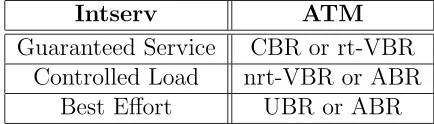
The services classes defined above can be mapped to ATM class quite easily. The

mapping is shown on table 2.1. In this table, the last line ‘Best Effort’ corresponds

to a regular unmanaged IP data transfer.

Intserv ATM

Guaranteed Service CBR or rt-VBR

Controlled Load nrt-VBR or ABR

[image:23.612.197.414.362.424.2]

Best Effort UBR or ABR

Table 2.1: Intserv/ATM Service Class mapping

2.4.2 Differentiated Services

In Intserv, the routers have to maintain information about all the flows which

are reserving resources at this node. If this method allows the network to provide

well-defined QoS, it does not scale well.

In Diffserv, the packets are classified at the edge of the network. They are given a

Differentiated Service (DS) codepoint. This codepoint is then used in the core of the

network to forward or drop the packets on a per-hop basis.

(24)

parts of the path are not diffserv-enabled, can inter-operate with other QoS

technolo-gies, and does not need to keep information about the flows.

These services are representatives of the efforts currently made to enable QoS

sup-port in IP, a protocol which was only designed to handle data transfers on unreliable

networks.

2.5 IP vs. ATM

About 8 years ago, ATM was seen as the future underlying technology for a lot of

different networks. However, the improvements in LANs domain made by Ethernet

technologies, in speed and in price, made ATM far less attractive for use in this

envi-ronment. The development of switched Ethernet has also been a major improvement

to Ethernet technology. With the recent innovation of Gigabit Ethernet, and soon 10

Gigabit Ethernet, ATM is even losing his advantages for use in MANs (Metropolitan

Area Networks). Nowadays, it is mostly used by telecom operators in network

back-bones or to extend local access.

However, ATM built-in traffic classes allow for an easy characterisation of the QoS

abilities offered to a customer by a telecom operator. Efforts are being made ([CGK02])

to improve this aspect of IP.

The importance of IP, with the use of the Internet, VPN, and VoIP technologies

is rising. The problem is that ATM is not designed to carry IP traffic very well. The

overhead added is about 15% of the data transmitted. The growing importance of

IP-based applications in the overall traffic is certainly another drawback for

ATM-based solutions. In [GW96], Gurski and Williamson report on the poor performance

of TCP over ATM, due to the poor interaction of two different designs, aimed at

(25)

2.6 NGN Planning

This section explains the example of Eircom migration plan ([Don01]). It is used

to illustrate the migration towards NGNs. This is just one possible example; almost

all telecommunication operators will have to create similar plans.

2.6.1 Current Network

The current network infrastructure used by Eircom is made of a telephony network

and an ATM network. This one represents the first step in Eircom migration to a

future multi-service network, carrying voice, IP traffic, legacy data, and eventually

leased lines. A smaller, separate ATM network has been deployed to support ADSL

deployment. The PSTN traffic is converted to ATM traffic by Media Gateways.

2.6.2 New Network Architecture

Today mobile telephony, PSTN/ISDN, Data/IP networks, Cable TV, and soon

wireless local loop, all have their own single-service networks.

The new network architecture will be made up of:

• a multi-service connectivity core,

• services and content providers running as applications on dedicated servers.

This is called application layer, and the services can be implemented by the

operator or by third-party service providers.

• multi-technology access systems connected to edge gateways, with control for

service access and connections across the core.

A detail view of the core of the NGN:

• The transmission is all optical, based on Dense Wavelength Division

(26)

• The transmission layer is based on IP routers, ATM switches or combinations of both.

• The core is interconnected to other services and other operators through media

gateways (ATM edge switches or IP edge routers).

Features of the core include: interoperability, scalability (capacity and

geographi-cally), reliability (Quality of Service or Guarantee of Service), adherence to standards

(to ensure good inter-working).

2.6.3 IP vs. ATM, Eircom Point of View

Currently, the preference of Eircom is for an ATM-based network. This

technol-ogy is favoured over IP, because of their existing ATM network, of the QoS built-in

guarantees of ATM, and its ability to carry high-quality voice traffic. This situation

represents well the point of view in the industry: the choice between ATM and IP

is driven by the existing network and the needs of the operators, no technology is

intrinsically better than the other for everything.

However, an overlay IP business network will be developed to complement the ATM

core. The core will be hybrid, between the two extremes, ‘all-ATM’ network or

‘IP-only’ network, supported by a new generation of ATM/IP integrated switches.

2.6.4 Migration Path

The evolution chosen by Eircom is a migration to a hybrid platform. This evolution

will be done in two phases:

1. Installation of IP routers in the core network. At this stage, different services

will be offered to customers: full QoS guarantee relying on the ATM network,

and lower quality, but cheaper, services running on top of the IP network.

2. Evolution of the core nodes to ATM/IP hybrids. Much of the development of

(27)

IP. This technology adds labels to IP headers to simplify routing. It provides a

good method to carry IP traffic over ATM and enable some sort of QoS support

in IP. Thus, the hybrid ATM/IP networks are referred as‘MPLS-based’

The migration path for telephony is still not clear. However, the general strategy is

to convert some PSTN switches to core gateways; the importance and the depth (in

the network hierarchy) of these changes is still to be determined.

2.7 Conclusion

IP and ATM both have valuable features to suggest they become the technology

of choice for telecom operators. However there is a common belief in the telecom

community that NGN will be made of all-IP multi-service networks ([Eri01b]).

The migration path is still not clear, and, depending on the existing infrastructure,

customers needs, and development strategy, the path to all-IP networks is likely to go

through an intermediate phase, where both technologies will be used. As described

in [SUOS01], design of multi-protocol routers may be needed to enable the use of

(28)

Chapter 3 Network Simulation

Preliminary work on this project suggested that a network simulator was needed

to provide the expected estimates of bandwidth requirements. This chapter provides

an overview of network simulation, with descriptions of the main simulators used, and

the different types of simulation possible. It also addresses the main concerns rising

when building a simulator.

3.1 Simulation in Network Research

As outlined in [BBE+_{99], network usage is evolving, and researchers need tools to}

test possible evolution scenarios: the protocols and standards are constantly changing,

as well as the usage of the existing network. The reasons for using simulation in general

also apply for network research:

• Modelling: when no applicable mathematical model of the system exits, or can

be evaluated, the simulation provides a numeric estimate of the characteristics

of the system. The goal may be to simulate reality, or to build a model and

simulate it.

• Planning: Simulation is used to review several options before deciding which

(29)

• The use of real testbeds is limited: usually the cost increases with the size, making simulation of wide-area networks difficult. Moreover reconfiguration of

the system is difficult and it’s impossible to reproduce exactly events showing a

random behaviour.

3.2 Network Simulators Overview

3.2.1 Simulation Abstraction Level

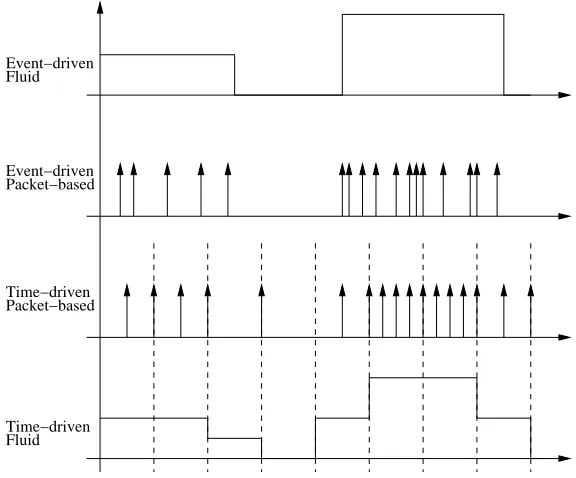
Several abstraction levels are used in network simulation. The next sections

de-scribes the main ones, while a graphical overview is given on figure 3.1.

Packet based simulation

In packet-based simulation, each packet1 _{transmitted on the network generates}

one event.

This method is the closest to real network behaviour. New protocols can be

imple-mented directly from their specification. However, the number of events generated

can be very high and make the problem uncomputable on major systems.

Nevertheless, event-driven packet-based simulation is the most common abstraction

used. [KS95] is an example of the use of packet-level simulation to simulate an ATM

network.

Fluid simulation

To overcome the computational barrier implicit in the previous methodology, fluid

simulation uses a different event model. Instead of generating one event for every

packet, the system is considered at an higher level. Data transmissions are considered

as flows which are described by their bit rate. The only events being considered are

the change of bit-rate for a given flow. A study of fluid simulation of ATM networks

(30)

is given in [KSCK96].

This method has two main drawbacks. The higher level of abstraction may need

some preliminary mathematical study before implementing a traffic type or a network

policy. The second drawback is that interactions between flows may increase the

amount of events generated drastically. This increase in the number of events caused

by interactions is called ripple effect in [LFG+_{01] and [KS95]. Liu, Figueiredo, Gua,}

Kurose and Towsley showed in [LFG+_{01] that, for scheduling policies such as single}

FIFO (First In - First Out) queueing, even on simple and small networks, more events

may be generated for fluid simulations than for a packet-based simulations. However,

for policies involving less interactions, such as GPS (Generalized Processor Sharing),

fluid simulation is still less expensive in computational power. It should also be noted

that doubling the bitrate of a source will cause the number of events in packet-based

simulation to double as well, while it will not have a significant impact on a fluid

simulation.

Hybrid model

Some simulators rely on a time-driven system rather than an event-driven one.

Such simulations are discrete: the time is split into small regular intervals. The

system state evolves at given time steps with this timescale influencing the precision

of the results. This differs significantly from the continuous simulators described

above.

Time-Stepped Hybrid Simulation (TSHS) [GGT00] is packet-based: packets

emit-ted during one time-step are grouped and assumed to be evenly spaced during this

period of time. This is called packet smoothing. [YG99] gives an overview of the

performance and precision of a time-driven fluid simulator: flows are fluid, however,

the rate remains constant during one time step.

The main advantage of time-driven simulation is the easy use of parallel

archi-tectures: all processors can easily agree on checkpoints, namely at the end of every

(31)

simu-lator.

Mixed mode

Other work ([YMTB01] has been done to extend fluid-modelling analysis to

packet-based simulation. The purpose of this method is to simulate some parts of the system

with a fluid flow-based analytical mode, and others with a discrete packet-based event

simulator, depending on which model is more appropriate to simulate a part of the

network. The simulator needs to provide the interface for translating flow model to

packet arrival, and the other way. The performance is increased when the flow model

is used to analyse sections of the network with heavy traffic, while a finner grained

packet-based simulation is used to analyse other parts.

Event−driven Fluid

Event−driven Packet−based

Time−driven

[image:31.612.162.450.341.580.2]

Time−driven Fluid Packet−based

(32)

3.2.2 Main Network Simulators

This section is a list of the most important network simulators. This list has been

gathered from several reviews, the most important being [Cha99] and [BBE+_{99]. This}

list is not exhaustive, as many network simulators have been developed over the past

15 years.

NS2

ns2 is part of the VINT (Virtual Inter-Network Testbed) project. It is a complete

network simulator, designed for test and validation of protocols. Written in C++,

with an interface in a language derived from Tcl, ns2 is freely available. A graphical

interface for analysing results is also available. One important feature of ns2 is the

ability to inject live traffic in the simulation. With a large library of protocols, ns2 has

been used widely, to investigate TCP behaviour, router queueing policies, multicast

transport, multimedia, wireless networking, application-level protocol, etc. A detailed

review of ns2 can be found in [BEF+_00].

PARSEC (GloMoSim)

PARSEC is developed by the Parallel Computing Laboratory at UCLA, as an

extension of the C programming language. The source code can be compiled for

dif-ferent parallel execution protocols, allowing very fast execution time.

Released in 1999, GloMoSim is a Parsec network simulation library designed to

sim-ulate wireless and ad hoc networks. It has since been extended by QualSim to handle

both wireless and wired networks.

OPNET

Founded in 1986, OPNET is a commercial product targeted in planning and

per-formance optimisation in communication networks. It is a discrete event network

(33)

MaRS

MaRS (Maryland Routing Simulator), from the University of Maryland, is a

discrete-event simulator designed to evaluate and to compare network routing

algo-rithms. The parameters are the actual network topology, traffic sources and routing

algorithms. MaRS has been used to evaluate and compare several next-hop routing

or link-state algorithms.

CLASS

CLASS stands for ConnectionLess ATM Services Simulator. It’s a time-driven,

synchronous simulator written in C. [MBD+_{95] provides a detailed review of the}

implementation and features of CLASS.

REAL

REAL provides a simulator interface to study the dynamic behaviour of flows and

congestion control schemes in packet-switched data networks. The simulation scenario

is input using a text file representing the network. Modules are provided to emulate

well-known flow control protocols and source types.

INSANE

Written in C++, INSANE (Internet Simulated ATM Networking Environment)

is a network simulator designed to test various IP-over-ATM algorithms with

realis-tic traffic loads derived from empirical traffic measurements. Internet protocols are

supported, including large subsets of IP, TCP, and UDP.

3.2.3 Alternatives to Network Simulators

Mathematical Modelling

(34)

ysed with such tool. However, Matlab may be used to generate code to model a part

of a system, which is then integrated into the simulator.

Petri Networks

Petri networks were first developed by Carl Adam Petri in 1962. Petri networks

represent a system using a state diagram, along with tokens. As stated in [Mur89]

by Murata, Petri networks are a graphical and mathematical tool “for describing and

studying information processing systems that are characterised as being concurrent,

asynchronous, distributed, parallel, nondeterministic, and/or stochastic”.

Some work have been done ([KK01], [MBGT97]) regarding the use of Petri nets for

modelling ATM traffic.

3.2.4 Summary

A wide range of tools have been developed to study and analyse networks. Each of

these tool has a set of targeted features, there is no general network simulator. Choices

and trade-offs have to be made regarding granularity, scalability, and specialisation

of the network simulator.

3.3 Technical Aspects

In this section, we will cover the major concerns to be addressed when writing a

simulator. This considerations, among many others, may be found in [LK00].

3.3.1 Future Event Set Management

An event-driven simulator has to maintain a list of future events. The management

of these events forms a significant part of the processing overhead in such a simulator.

[MS81] and [LK00] provide an overview of such algorithms:

(35)

performance is usually poor, because the insertion of a new event has to be

made by linear search. However, retrieving the first element (i.e. the next event

at a current time) is fast.

• Indexed list structures: maintaining a set of intermediate pointers can speed up

the process of inserting a new event at the right place in the list. The

mainte-nance of these pointers does not usually had a lot of overhead on the

computa-tional effort. At first the event to be inserted is compared to the intermediate

pointers, then a linear search is started from the appropriate pointer.

• Other data structures: non-linear structures such as binary trees and heaps may

be used. These structures may be complex to implement, and their efficiency

depends on the distribution of the event set, even if the performance are better

than the previous method in general.

These algorithms are not fundamentally different from the well-known sort algorithms.

However, the distribution across time of the event set has an impact on the

perfor-mances, and has to be taken into consideration.

3.3.2 Random Number Generation

[LK00] emphasises the importance of randomness in simulation. The goal is to

provide a realistic and accurate numeric estimation of a system, and as most elements

involve random behaviour, a random number generator is needed. However, the final

simulation results must be obtained by running several simulations using different

sequences of random numbers. These sequences must be truly random, and be

un-correlated with each other.

The random variables are generated in two steps:

• a pseudo-random number generator is used to generated one or more uniform

variables over [0,1]. The main characteristic of the pseudo-random number

(36)

(seed) will produce the same results, and after a certain number of generations,

the generator will be re-initialised by producing the initial seed. This may seem

to be a major drawback for these generators. However, this has been studied

in depth, and it has been proved that, provided the period is very long, the

sequence is random to all intends and purposes.

• the variable(s) generated are then used to produced a random variate

corre-sponding to the appropriate random distribution. The complexity of this

gen-eration and the number of variates from _U[0,1] needed may vary, depending on

the complexity of the distribution.

3.4 Conclusion

This chapter provides an overview of the preliminary work carried out prior to the

implementation of the network simulator layer of the planning tool. We reviewed the

motivation for writing a simulator, along with details of how network simulators are

implemented. We also looked at existing network simulators.

The actually software development is described in the next three chapters. Chapter 6

(37)

Chapter 4 Design & Implementation

This chapter details the work done in the first phase of the project: specification

of the software to be implemented, and design of the core parts of the tool.

A detailed view of the re-implementation of [Hov01] and the actual implementation

of the network simulator will be studied in the following two chapters.

4.1 Introduction

4.1.1 Specifications

The tool was developed in two phases:

Step 1 Design and implementation of the network model (section 4.3); implementation

of algorithms to compute network bandwidth usage.

The algorithms are described in the next section, while a detailed analysis is

given in section 7.2.4.

Step 2 Implementation of a network simulator on top of the network structure

devel-oped in the first step.

This additional layer was needed to provide additional metrics, which could not

(38)

For the simulator (step 2), metrics are provided to measure the following:

• Bandwidth used (bitrate),

• Packet loss ratio,

• Delay,

• Maximum bandwidth used for a link.

Measurements of the continuous evolution of the bitrate through time are available,

along with the average value for all measurements of interest, which is produced at

the end of the simulation. The tool is able to launch several simulations varying one

or several parameters (e.g. buffer size, switch service rate). This allows for easy study

of the impact of these parameters on the system behaviour. The random number

sequence used will be generated with the same seed across all of these simulations to

allow for comparison. As stated in [LK00], one should not rely on one simulation.

Several simulations should be used to ensure that the average values are converging.

The C++ programming language was used. As speed was a major drawback of

the previous implementation, a special effort was made to optimise the algorithms

used in this tool. Speed of the program was considered when making choices in the

design phase, and during the implementation. However, some non-optimal solutions

have been implemented because of the lack of time. For example, the support for

parallel execution has been neglected because of its complexity, in spite of the fact

that this technique has a very important effect on the execution time.

4.1.2 Common Aspects

In the next sections, we will describe the aspects which are common to the main

parts of the tool.

(39)

the bandwidth or the simulation. This is done using a simple shortest-path

algorithm.

• Network model: The network infrastructure is described in same way for both stages of the implementation. The information which is provided to the

simu-lator is more complex, as both source model and switch technology impact on

the results.

• Scripting language: The interface instantiates objects representing the network elements and agents. An extended version has been developed to cover the

subclasses needed for the second version of the tool.

• Environment: All the objects are stored in a common environment. This al-lows for ease of instantiation, as well as common object reference, in the input

interface.

4.2 Routing

The routing is done using a shortest-path algorithm. The links can be weighted

either by their respective delays or equally.

This algorithm is complex (O(S3_{), where} _S _{is the number of nodes). However, it}

computes all the paths, which are needed for the bandwidth requirement computation.

The main drawback of this method is that it rules out the possibility of enabling

dynamic routing.

4.2.1 Notation

The following notation is used in the next section:

• S is the number of nodes, and M the number of links in the environment,

(40)

• for ni, nj ∈ N, P(ni, nj) is the path from node ni to node nj, and d(ni, nj) is

the weighted length of this path,

• for a link l ∈ L, na(l) and nb(l) are the two nodes at each end of the link (we

assume thatna(l)6=nb(l).

4.2.2 Algorithm

The routing algorithm involves three steps. The first two initialise the algorithm.

Step one initialises all distances to infinity, except for one node to itself where the

distance is 0. There are no paths specified. The second step initialises the distance

and the path for each direct connections.

Finally, the third step iterates through all the paths to check if the use of an

inter-mediate node can shorten the path. If it does, the path is modified accordingly.

1. for allni ∈N

for allnj ∈N

if i=j,     

P(ni, nj) = [∅], P(nj, ni) = [∅]

d(ni, nj) = 0, d(nj, ni) = 0

else d(ni, nj) = ∞,d(nj, ni) =∞

2. for alll ∈L

d(na(l), nb(l)) =W(l),

d(nb(l), na(l)) =W(l),

P(na(l), nb(l)) = [l],

P(nb(l), na(l)) = [l].

3. for allnk ∈N

for allni ∈N

for allnj ∈N

if d(ni, nj)> d(ni, nk) +d(nk, nj) then

(41)

4.3 Network Model

4.3.1 Model

The network is represented as a set of nodes bounded by links. The agents are the

sources, switches (or routers), and sinks on the network. At least one agent has to be

mapped to every node. Only one switch can be mapped to a given node. Subclasses

of Source represent different traffic models, while subclasses of Switch represent

different scheduling policies. Note that the subclasses of Source and Switch are not

relevant for the bandwidth calculation algorithm. Details about the properties of

these classes are given in the following section.

4.3.2 Class Hierarchy

Element

• Agent

– Sink

– Source

∗ SourceCBR

∗ SourceMMP

∗ SourceOnOff

– Switch

∗ PriorityScheduler

∗ QueueMultiplexer

∗ SingleFifo

• Link

(42)

• Value

– Const

– Var

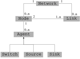
4.3.3 Class Diagram

The class diagram is given on figure 4.1. This diagram means that a network is

composed of nodes and links. A link is associated with two different nodes. Traffic

agents (sources, sinks and switches) have to be attached to each nodes.

Network

Node

Agent

Switch

Link

Sink

Source

0..n

1

2

1 0..n

0..n

[image:42.612.134.477.265.518.2]

1..n

Figure 4.1: Class Diagram

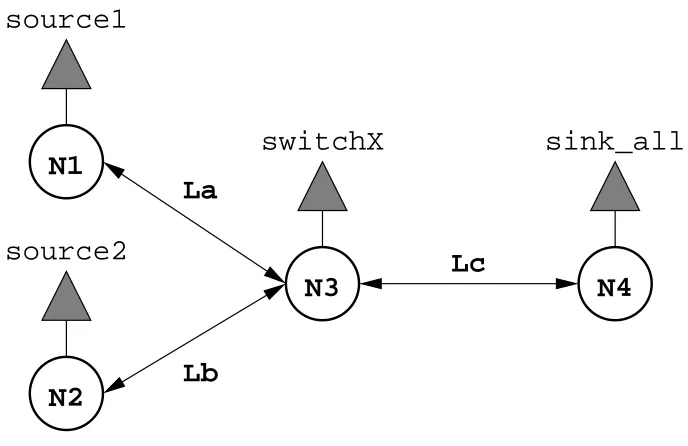
4.3.4 Example

A sample network is shown on figure 4.2. It consists of four nodes,N = (n1, n2, n3, n4),

and 3 links, L= (la, lb, lc). Two sources, source1and source2 are mapped to nodes

n1 and n2 respectively. The traffic from these sources is going through the switch

(43)

source2

switchX

sink_all

Lc

La

Lb

source1

N1

N2

[image:43.612.134.478.56.279.2]

N3

N4

Figure 4.2: Example Network

4.4 Interface

The interface is text-based. A graphical interface had been planned in the initial

proposal, but efforts have concentrated on improving the tool’s features. However,

the system is designed to allow an easy implementation of a GUI on top of the current

script based interface.

4.4.1 Input Scripting language

Syntax

Scripts are used to provide input to the simulator. The core set of command is:

• new <class> <object name> [<param1> ...]: create a new instance ofclass

namedobject name. The parameters are optional or mandatory, depending on

the class instantiated.

• set <object name> <property> <value>: set property of the object named

(44)

process the rest of the calling script file. This can be done recursively. This

feature allows easier configuration of very similar network scenarios.

• compute bw: compute the bandwidth required on every link on the given net-work.

• run sim: start the simulation.

• print env: print the environment (debug only).

Lines beginning with # are considered as comments. If the tool is called without any

parameter file, a shell will be open and the user will be prompted for commands line

by line.

Complete syntax and examples are given in sections 5.3 and 6.2.

Example

This is the script used to instantiate the objects representing the network used as

an example in section 4.3.4 (figure 4.2).

# network infrastructure

new node N1

new node N2

new node N3

new link La N1 N3

new link Lb N2 N3

new link Lc N3 N4

# traffic agents

(45)

new switch switchX N3

new const bitrate 100.0

new source source1 N1

set source1 rate bitrate

set source1 dest sink_all

# bandwidth

compute_bw

4.4.2 Output

Different types of output files are generated, depending on the functionality used:

• Bandwidth usage: a file containing a tab-separated array is produced. For

every link, the following data is given: link name, average bitrate, bandwidth

required on PSTN networks, bandwidth required on ATM networks, difference

in percentage. An example is given in section 7.2, table 7.2.

• Simulation: The evolution of some network element values is stored in a file in

Gnuplot format. Only the values specified in the input script will be plotted.

The main drawback of this strategy is that the simulation needs to be re-run if

another value needs to be studied. On the other hand, writing this files adds

a lot of overhead on computation, and plotting all the values is certainly not a

(46)

4.5 Environment

4.5.1 Hash Table Structure

Every object instantiated by a script has an unique name. For ease of retrieval,

the environment is represented using an hash table, with the object name used as a

key. The hash value is computed using this function, to ensure maximum dispersion

of the values across the table:

int hash_value (string name) {

int ret = 0;

for (unsigned int i=0; i<name.length(); i++) {

ret += name[i] * name[i] * (i+1);

}

return ret % ENV_DEFAULT_SIZE;

}

4.5.2 Variables

For research purposes, the ability to run several simulations changing a few

pa-rameters, and keeping the same set of random seeds for the random-driven source is

vital.

To allow for study of the impact of one or several parameters, the following strategy

is used. All the numeric object properties, which on the lowest level as considered as

C++ double, are instantiations of one of the subclasses of the class Value. There is

two subclasses of Value: Const and Var.

Subclass Const

This is used to represent a value which will not change across the simulations.

(47)

to update this script (e.g. the delays associated with all the links). When a value is

expected by the script interpreter, a literal number can be inputed. In this case, a

Const object is instantiated. Its name is the string representation of the number.

Subclass Var

This subclass is used to run several simulations with the object of this class

varying its value. The syntax to instantiate such objects in the script is: new var

<name> <init> <end> <increment>. The value is started at <init>, incremented

by <increment>, while the value is equal to or lower than <end>.

If multiple Var objects are instantiated, all the possible combinations will be run.

4.6 Chapter Summary

In this section we have reviewed all the abstraction levels and interfaces used in the

current implementation. The common features are: routing, network infrastructure

model, script interpretation, and variables environment. All these features have been

developed for the bandwidth computation, and have been extended if needed for the

(48)

Chapter 5 Bandwidth Computation

5.1 Description

In this chapter, we will review the features of the re-implementation of Hovland’s

work. The results are an estimation of the gain in bandwidth requirements obtained

with the migration from a telephony PSTN-based network to an ATM-based network.

The next sections describe the source model and the algorithms used for bandwidth

gain computation. A detailed analysis is given in section 7.2.4.

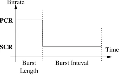
5.2 Traffic Source Model

We are considering three different types of traffic: High Quality voice, Low Quality

voice, and Video. The traffic is described using the ATM specification. This kind of

traffic is bursty: during some time, the bitrate is Peak Cell Rate (PCR), and then is

reduced to Sustainable Cell Rate (SCR). Such traffic is described on figure 5.1, and

(49)

PCR

SCR

Burst Length

Burst Inteval Bitrate

[image:49.612.134.447.59.431.2]

Time

Figure 5.1: Traffic types

Traffic PCR SCR Burst Burst AAL

Type kb/s kb/s Length Interval

HQ Voice 64 64 * * AAL1

LQ Voice 64 16 30 300 AAL2

Video 256 32 30 300 AAL2

Table 5.1: Traffic Types

5.3 Input Script

5.3.1 Syntax

To set up the configuration, the network topology needs to be defined, using Node

and Link objects. The syntax to define those is:

• new node <name>,

• new link <name> <node1> <node2>.

Then agents are mapped to the nodes. For bandwidth computation, we do not

con-sider traffic policies, so all the nodes are implicitly used as a switch, there is no need

to instantiate Switch objects. Source and Sink objects are defined by:

• new source <name> <node>,

set <name> rate <value>,

[image:49.612.208.407.60.186.2]

(50)

• new sink <name> <node>.

Several sources can have the same sink as a destination.

Some choices have been made regarding the parameters which should be included

in the instantiation of an object (command new) or should be set after (command

set). In an early version of the scripting language, all the parameters had to be set.

However, this solution tends to make the scripts long. On the other hand, the numbers

of parameters on the new command line has to stay small, as too many parameters

tends to be confusing. Some parameters are mandatory on the new command line,

while others are to be set; the general criteria is to include in the command line

parameters which are used in both versions of the tool.

5.3.2 Example

The example given in section 4.4.1 is actually a valid script for bandwidth

com-putation:

# network infrastructure

new node N1

new node N2

new node N3

new link La N1 N3

new link Lb N2 N3

new link Lc N3 N4

# traffic agents

new sink sink_all N4

(51)

new const bitrate 100.0

# bandwidth

compute_bw

5.4 Algorithm

The first step computes the exact traffic mix on all links, while the second step

computes the bandwidth needed for PSTN and ATM-based networks.

Step 1 for all sources

for all links in path (source, sink)

add (traffic type, rate)

Step 2 for all links

compute bandwidth (PSTN)

(52)

Chapter 6 Network Simulator

6.1 Implementation

This chapter describes the implementation of a simple network simulator. This

functions on top of the previously described tool.

A fluid, event-driven simulator has been used. This type of simulator has been chosen

because it provides a good estimation of the metrics needed, it is usually faster than

packet-based simulation, and because we only need estimates rather than exact values.

This chapter gives an overview of extensions to the existing program, and of the key

algorithms used at simulation run-time.

6.2 Scripting Language Extension

The scripting language has been extended to integrate the new features.

Network Agents

The newcommands forsourceand switchhave been updated. As the sinkclass

is passive and used only to collect data, there was no need to alter this.

new <source type> <name> [<parameters>...] <rate>. There is three different

(53)

to the three traffic source models described in section 6.4. The command lines are:

• new source cbr <name> <bitrate>,

• new source mmp <name> <lambda> <mu> <off rate> <on rate>,

• new source type <name> <lambda> <mu> <N> <beta>

For all the sources, two additional parameters have to be set: start and stop, with

the starting and stopping times for the source. When a priority scheduler is involved,

the parameter priority has to be set.

For the subclasses of Switch described in section 6.5, the syntax is:

• new <switch type> <name> <service rate> <buffer size>,

where <switch type> must be fifo, gps, or prio.

Output Control

The output is simple text files which can be used as input for the Gnuplot program.

As writing to these files take a significant time, the user needs to specify precisely

which graph should be plotted.

There is two different types of graphs generated by the tool: evolution of bitrate of

an agent through time, and loss and delay for a source, as a function of a system

parameter.

The first option allows multiple agent bitrates to be plotted on the same graph. This

is done using the class monitorand the command plot as follow:

new monitor <name>

plot <agent> <monitor>

The rate value plotted depends on the agent type:

• source: output bitrate,

(54)

The metrics for the flows (identified by a source) are produced using:

graph <source name> <x var> [<y var>],

where x var and y var are the name of two Var objects. y var is optional. If it is

used, a 3D graph will be plotted.

6.3 Events Scheduling

This section outlines the events scheduling algorithm, a key part of the network

simulator.

6.3.1 Event

Class

Class Hierarchy

Event

• BufferEvent

• DepartureEvent

• FlowEvent

• SourceEvent

Description

Four different types of event are implemented:

• Source state: This event represents a change in a source bitrate. Only one event

of this type is scheduled for each source, to keep the event list small.

• Flow bitrate: represents a change in a flow arrival bitrate at one node.

(55)

• Buffer state: as the filling status of the buffer influences the behaviour of the system, the simulator needs to schedule the changes on the buffer status.

The event propagation mechanism is demonstrated in next section.

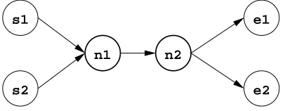
6.3.2 Example

The network described in figure 6.1 is used in this example.

n1 n2

e1

e2 s1

[image:55.612.206.409.226.305.2]

s2

Figure 6.1: Example Network

This network consists in two sources,s1ands2, sending data respectively to the sinks

e1 ande2. All the traffic goes through the switchesn1 andn2. All the links have the

same bandwidth b and propagation time θ. s1 sends cells between t0 and t2, and s1

between t1 and t3. We have t0 < t1 < t2 < t3 and ti >> θ, with i ∈ {0,1,2,3}. The

second assumption is not needed by the simulator, but it makes this example clearer.

During their transmission time, the two sources are sending data at the same bit rate

0.6b. This value is used to outline the buffer state management: whens1 and s2 are

sending data together, betweent1 and t2, the dimension of the linkn1-n2is too small

to handle a bitrate of 1.2b.

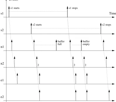
Figure 6.2 represents the relationships between events. Arrows are representing

events, a dashed line between eventsA and B, withtA< tB, means B is spawned by

A; 2 at the base of an arrow means two simultaneous events. Uncommented events

(56)

s1

s2

n1

n2

e1

e2

2 2

Events

s1 starts s1 stops

s2 starts s2 stops

full

buffer buffer

empty

Time

[image:56.612.106.503.189.538.2]

2

(57)

6.3.3 Future Events List Management

The strategy described in the previous section allows for the event list to stay

relatively small. At any given time, there is usually one event per source for the next

state transition, and at most one more event for the propagation of the last change

through the path. At node level, the next change in the status of the buffer (full or

empty) may be scheduled if necessary.

Maintaining a small and relatively constant event list over time is good for

perfor-mance and memory usage. As most of events only spawn one other event of the same

type, memory used for this event can be recycled, instead of being freed and

real-located. The event list needs to be, and remain sorted. Minimising its size is quite

important, even if there are algorithms which are better than linear search for this

task.

In this implementation, three pointers to relevant elements of the list are kept up to

date: the first element, the last element and the last inserted element. When an

ele-ment has to be inserted or updated, its timestamp is compared to these three values.

It may be inserted before the first element, after the last one, or in between using a

linear search starting from the first element or from the last inserted element.

6.4 Traffic Models

Every source has a traffic model attached. All the models used in this simulator

should be described as a series of constant bitrate traffic flows. While the source is

evolving through states, the bitrate during an individual state should stay constant.

However, the length of the state and the bitrate associated may be determined by

random values. Figure 6.3 represents a source going through five different states

during the simulation time.

This section contains a detailed list of the available traffic models. The following

(58)

Bitrate

1 2 3 4 5 Time

[image:58.612.178.432.76.187.2]

End of simulation

Figure 6.3: Example Source Bit Rate

function of time. This feature has been very useful for debugging purposes, but the

significant results are usually the average values over one simulation.

The different traffic models have been selected from several surveys ([JMW96], [MM99],

[RK96]). The traffic models used were chosen because they are easy to implement,

and are sufficient to simulate various traffic types.

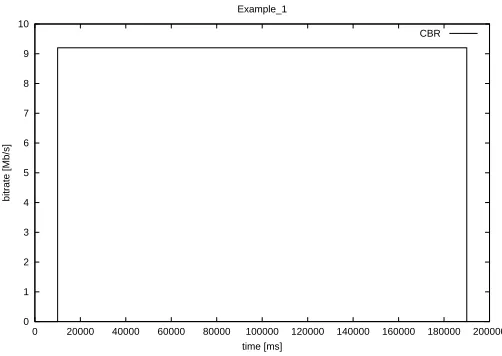
6.4.1 Constant Bit Rate

This model is used to simulate constant traffic, such as that described by the CBR

traffic class of ATM. A sample is given in figure 6.4. This traffic was not used much

during the detailed analysis phase of the project (chapter 7), but it was used early

in the implementation process for debugging purposes, as it represents the simplest

source, with only one state. This source model is only defined by the bitrateβ.

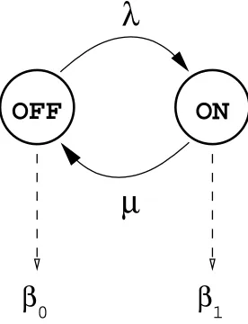
6.4.2 Markov-Modulated Rate Process

For the sources of this type, the underlying mechanism is a Markov chain with N

states. The bitrate at any given time is the state index multiplied by the bitrate per

state value, β: at state n, the bitrate of the source isn_×β.

λ and µ represent the parameters of the exponential probability law, which define

respectively the probability of moving from state n to n + 1, and from state n to

Modelling and Planning the Migration for Next Generation Networks