Unsupervised Learning on an Approximate Corpus

Unsupervised Learning on an Approximate Corpus

Jason Smith and Jason Eisner Center for Language and Speech Processing

Johns Hopkins University

3400 N. Charles St., Baltimore, MD 21218, USA {jsmith,jason}@cs.jhu.edu

Unsupervised learning techniques can take advan-tage of large amounts of unannotated text, but the largest text corpus (the Web) is not easy to use in its full form. Instead, we have statistics about this corpus in the form of n-gram counts (Brants and Franz, 2006). Whilen-gram counts do not directly provide sentences, a distribution over sentences can be estimated from them in the same way that n -gram language models are estimated. We treat this distribution over sentences as anapproximate cor-pus and show how unsupervised learning can be performed on such a corpus using variational infer-ence. We compare hidden Markov model (HMM) training on exact and approximate corpora of vari-ous sizes, measuring speed and accuracy on unsu-pervised part-of-speech tagging.

1 Introduction

We consider the problem of training generative mod-els on very large datasets in sublinear time. It is well known how to train an HMM to maximize the like-lihood of a corpus of sentences. Here we show how to train faster on a distribution over sentences that compactly approximates the corpus. The distribu-tion is given by an 5-gram backoff language model that has been estimated from statistics of the corpus. In this paper, we demonstrate our approach on a traditional testbed for new structured-prediction learning algorithms, namely HMMs. We focus on unsupervised learning. This serves to elucidate the structure of our variational training approach, which stitches overlapping n-grams together rather than treating them in isolation. It also confirms that at least in this case, accuracy is not harmed by the key approximations made by our method. In future, we hope to scale up to the Google n-gram corpus (Brants and Franz, 2006) and learn a more detailed, explanatory joint model of tags, syntactic dependen-cies, and topics. Our intuition here is that web-scale data may be needed to learn the large number of lex-ically and contextually specific parameters.

∗

Work was supported in part by NSF grant No. 0347822.

1.1 Formulation

Let w (“words”) denote an observation sequence, and let t (“tags”) denote a hidden HMM state se-quence that may explain w. This terminology is taken from the literature on inducing part-of-speech (POS) taggers using a first-order HMM (Merialdo, 1994), which we use as our experimental setting.

Maximum a posteriori (MAP) training of an HMMpθseeks parametersθto maximize

N·X

w

c(w) logX

t

pθ(w,t) + log Prprior(θ) (1)

where c is an empirical distribution that assigns probability 1/N to each of the N sentences in a training corpus. Our technical challenge is to gen-eralize this MAP criterionto other, structured dis-tributionscthat compactly approximate the corpus.

Specifically, we address the case wherecis given by anyprobabilistic FSA, such as abackoff lan-guage model—that is, a variable-order Markov model estimated from corpus statistics. Similar sen-tenceswshare subpaths in the FSA and cannot eas-ily be disentangled. The support ofcis typically infi-nite (for a cyclic FSA) or at least exponential. Hence it is no longer practical to compute the tagging distri-butionp(t|w)for each sentencewseparately, as in traditional MAP-EM or gradient ascent approaches. We will maximize our exact objective, or a cheaper variational approximation to it, in a way that cru-cially allows us to retain the structure-sharing.

1.2 Motivations

Why train from a distribution rather than a corpus? First, the foundation of statistical NLP is distribu-tions over strings that are specified by weighted au-tomata and grammars. We regard parameter estima-tion from such a distribuestima-tion c (rather than from a sample) as a natural question. Previous work on modeling c with a distribution from another fam-ily was motivated byapproximating a grammar or

model rather thangeneralizing from a dataset, and hence removed latent variables while adding param-eters (Nederhof, 2000; Mohri and Nederhof, 2001; Liang et al., 2008), whereas we do the reverse.

Second, in practice, one may want to incorporate massive amounts of (possibly out-of-domain) data in order to getbetter coverageof phenomena. Mas-sive datasets usually require a simple model (given a time budget). We propose that it may be possible to use a lot of dataanda good model by reducing the accuracy of the data representation instead. While training will become more complicated, it can still result in an overall speedup, because a frequent 5-gram collapses into a single parameter of the esti-mated distribution that only needs to be processed once per training iteration. By pruning low-count

n-grams or reducing the maximumnbelow 5, one can further increase data volume for the fixed time budget at the expense of approximation quality.

Third, one may not have access to the original corpus. If one lacks the resources to harvest the web, the Google n-gram corpus was derived from over a trillion words of English web text. Privacy or copyright issues may prevent access, but one may still be able to work withn-gram statistics: Michel et al. (2010) used such statistics from 5 million scanned books. Several systems usen-gram counts (Bergsma et al., 2009; Lin et al., 2009) or other web statistics (Lapata and Keller, 2005) as features within a classifier. A large language model fromn -gram counts yields an effective prior over hypothe-ses in tasks like machine translation (Brants et al., 2007). We similarly construct ann-gram model, but treat it as the primarytrainingdata whose structure is to be explained by the generative HMM. Thus our criterion does not explain then-grams in isolation, but rather tries to explain the likely full sentences wthat the model reconstructed from overlappingn -grams. This is something like shotgun sequencing, in which likely DNA strings are reconstructed from overlapping short reads (Staden, 1979); however, we train an HMM on the resulting distribution rather than merely trying to find its mode.

Finally, unsupervised HMM training discovers la-tent structure by approximating an empirical distri-butionc(the corpus) with a latent-variable distribu-tionp(the trained HMM) that has fewer parameters. We show how to do the same where the distribution

c is not a corpus but a finite-state distribution. In general, this finite-stateccould represent some so-phisticated estimate of thepopulationdistribution, using shrinkage, word classes, neural-net predictors, etc. to generalize in some way beyond the training sample before fitting p. For the sake of speed and clear comparison, however, our present experiments takecto be a compact approximation to thesample

distribution, requiring onlyn-grams.

Spectral learning of HMMs (Hsu et al., 2009) also learns from a collection ofn-grams. It has the striking advantage of converging globally to the true HMM parameters (under a certain reparameteriza-tion), with enough data and under certain assump-tions. However, it does not exploit context beyond a trigram (it will not maximize, even locally, the likelihood of a finite sample of sentences), and can-not exploit priors or structure—e.g., that the emis-sions are consistent with a tag dictionary or that the transitions encode a higher-order or factorial HMM. Our more general technique extends to other latent-variable models, although it suffers from variational EM’s usual local optima and approximation errors.

2 A variational lower bound

Our starting point is the variational EM algorithm (Jordan et al., 1999). Recall that this maximizes a lower bound on the MAP criterion of equation 1, by bounding the log-likelihood subterm as follows:

logP

tpθ(w,t) (2)

= logP

tq(t)(pθ(w,t)/q(t))

≥P

tq(t) log(pθ(w,t)/q(t))

=Eq(t)[logpθ(w,t)−logq(t)] (3) This use of Jensen’s inequality is valid for any distri-butionq. As Neal and Hinton (1998) show, the EM algorithm (Dempster et al., 1977) can be regarded as locally maximizing the resulting lower bound by alternating optimization, whereq is a free parame-ter. The E-step optimizesq for fixedθ, and the M-step optimizesθfor fixedq. These computations are tractable for HMMs, since the distribution q(t) =

factorial HMMs and Bayesian HMMs in which an expectation underpθ(t| w)involves an intractable sum. In this setting, one may use variational EM, in which q is restricted to some parametric family qφ that will permit a tractable M-step. In this case the E-step chooses the optimal values of thevariational parametersφ; the inequality is no longer tight.

There are two equivalent views of how this pro-cedure is applied to a trainingcorpus. One view is that the corpus log-likelihood is just as in (2), where w is taken to be the concatenation of all training sentences. The other view is that the corpus log-likelihood is a sum over many terms of the form (2), one for each training sentencew, and we bound each summand individually using a differentqφ.

However, neither view leads to a practical imple-mentation in our setting. We can neither concatenate all the relevantwnor loop over them, since we want the expectation of (2) under some distributionc(w)

such that{w : c(w) > 0}is very large or infinite. Our move is to makeq be aconditionaldistribution

q(t | w)that applies to allwat once. The follow-ing holds by applyfollow-ing Jensen’s inequality separately to eachwin the expectation (this is valid since for eachw,q(t|w)is a distribution):

Ec(w)log

P

tpθ(w,t) (4)

=Ec(w)log

P

tq(t|w)(pθ(w,t)/q(t|w))

≥_Ec(w)P

tq(t|w) log(pθ(w,t)/q(t|w))

=Ecq(w,t)[logpθ(w,t)−logq(t|w)] (5) where we use cq(w,t) to denote the joint distribu-tionc(w)·q(t |w). Thus, just ascis our approx-imate corpus,cq is our approximatetaggedcorpus. Our variational parametersφwill be used to param-eterize cq directly. To ensure that cqφ can indeed be expressed asc(w)·q(t | w), making the above bound valid, it suffices to guarantee that our varia-tional family preserves the marginals:

(∀w)P

tcqφ(w,t) =c(w)

3 Finite-state encodings and algorithms

In the following, we will show how to maximize (5) for particular families of p, c, andcq that can be expressed using finite-state machines (FSMs)— that is, finite-state acceptors (FSAs) and transducers (FSTs). This general presentation of our method en-ables variations using other FSMs.

A path in an FSA accepts a string. In an FST, each arc is labeled with a “word : tag” pair, so that a path accepts a stringpair(w,t)obtained by respec-tively concatenating the words and the tags encoun-tered along the path. Our FSMs are weighted in the

(+,×)semiring: the weight of any path is the prod-uct (×) of its arc weights, while the weight assigned to a string or string pair is the total weight (+) of all its accepting paths. An FSM isunambiguousif each string or string pair has at most one accepting path.

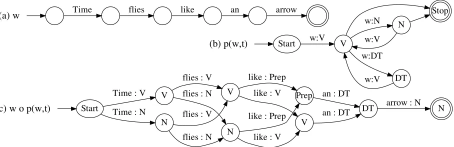
Figure 1 reviews how to represent an HMM POS tagger as an FST (b), and how composing this with an FSA that accepts a single sentence gives us the familiar HMM tagging lattice as an FST (c). The forward-backward algorithm sums over paths in the lattice via dynamic programming (Rabiner, 1989).

In section 3.1, we replace the straight-line FSA of Figure 1a with an FSA that defines a more gen-eral distribution c(w) over many sentences. Note that we cannot simply use this as a drop-in replace-ment in the construction of Figure 1. That would correspond to running EM on a single but uncer-tain sentence (distributed asc(w)) rather than a col-lection of observed sentences. For example, in the case of an ordinary training corpus ofN sentences, the new FSA would be a parallel union (sum) of

N straight-line paths—rather than a serial concate-nation (product) of those paths as in ordinary EM (see above). Running the forward algorithm on the resulting lattice would compute Ec(w)

P

tp(w,t),

whose log is logEc(w)

P

tp(w,t) rather than our

desired Ec(w)log

P

tp(w,t). Instead, we use cin

section 3.2 to construct a variational familycqφ. We then show in sections 3.3–3.5 how to compute and locally maximize the variational lower bound (5).

(a) w Time flies like an arrow

(b) p(w,t) Start w:V V

Stop N

w:N

DT w:DT

w:V

w:V

(c) w o p(w,t) Start

V Time : V

N Time : N

V flies : V

N flies : N

flies : V

flies : N

Prep like : Prep

V like : V

like : Prep

like : V

DT an : DT

an : DT arrow : N N

Figure 1: Ordinary HMM tagging with finite-state machines. An arc’s label may have up to three components: “word:tag / weight.” (Weights are suppressed for space. State labels are not part of the machine but suggest the history recorded by each state.) (a)wis an FSA that generates the sentence “Time flies like an arrow”; all arcs have probability 1. (b)p(w,t)is an FST representing an HMM (many arcs are not shown and words are abbreviated as “w”). Each arc w:tis weighted by the product of transition and emission probabilities,p(t| previoust)·p(w| t). Composing (a) with (b) yields (c), an FST that encodes the joint probabilitiesp(w,t)of all possible taggings of the sentencew.

of weight 0 can be omitted from the FSA.1

To estimate a conditional probability like c(h |

defg)above, we simply take an unsmoothed ratio of twon-gram counts. This ML estimation means that

cwill approximate as closely as possible the train-ing sample from which the counts were drawn. That gives a fair comparison with ordinary EM, which trains directly on that sample. (See discussion at the end of section 1.2 for alternatives.)

Yet we decline to construct a full 5-gram model, which would not be as compact as desired. A col-lection of all web 5-grams would be nearly as large as the web itself (by Zipf’s Law). We may not have such a collection. For example, the Googlen-gram corpus version 2 contains counts only for 1-grams that appear at least 40 times and 2-, 3-, 4-, and 5-grams that appear at least 10 times (Lin et al., 2009).

1

The FSA’s initial state is the unigram history#, and its final states (which have no outgoing arcs) are the other states whose

n-gram labels end in#. Here#is a boundary symbol that falls between sentences. To compute the weighted transitions, sen-tence boundaries must be manually or automatically annotated, either on the training corpus as in our present experiments, or directly on the trainingn-grams if we have only those.

To automatically find boundaries in an n-gram collection, one could apply a local classifier to eachn-gram. But in princi-ple, one could exploit more context and get a globally consistent annotation by stitching then-grams together and applying the methods of this paper—replacingpθwith an existing CRF sen-tence boundary detector, replacingcwith a document-level (not sentence-level) language model, and optimizingcqφto be a ver-sion ofcthat is probabilistically annotated with sentence bound-aries, which yields our desired distribution over sentences.

Instead, we construct a backoff language model. This FSA has one arc for each n-gram in the col-lection. Our algorithm’s runtime (per iteration) will be linear in the number of arcs. If the 5-gramdefgh is not in our collection, then there can be noh arc leavingdefg. When encounteringhin statedefg, the automaton will instead take afailure arc(Allauzen et al., 2003) to the “backoff state” efg. It may be able to consume thehfrom that state, on an arc with weightc(h |efg); or it may have to back off further tofg. Each state’s failure arc is weighted such that the state’s outgoing arcs sum to 1. It is labeled with the special symbolΦ, which does not contribute to the word string accepted along a path.

We take care never to allow backoff to the empty state ,2 since we find that c(w) is otherwise too coarse an approximation to English: sampled sen-tences tend to be disjointed, with some words gener-ated in complete ignorance of their left context.

3.2 The variational distributioncq(w,t)

The “variational gap” between (4) and (5) is

Ec(w)KL(q(t|w)||pθ(t|w)). That is, the bound is good ifq does a good job of approximating pθ’s tagging distribution on a randomly drawn sentence.

Note thatn−1is the order of ourn-gram Markov

2

modelc(w)(i.e., each word is chosen given the pre-viousn−1words). Letnp−1be the order of the HMMpθ(w,t)that we are training: i.e., each tag is chosen given the previousnp−1tags. Our experi-ments takenp = 2(a bigram HMM) as in Figure 1.

We will takeqφ(t|w)to be aconditional Markov

modelof ordernq−1.3 It will predict the tag at po-sitioniusing a multinomial conditioned on the pre-cedingnq−1tags and on the wordn-gram ending at positioni(wherenis as large as possible such that thisn-gram is in our training collection). φis the collection of all multinomial parameters.

Ifnq =np, then our variational gap can be made 0 as in ordinary non-variational EM (see section 3.5). In our experiments, however, we save memory by choosingnq = 1. Thus, our variational gap is tight to the extent that a word’s POS tag under the model

pθis conditionally independent of previous tags and the rest of the sentence,given ann-word window.4 This is the assumption made by local classification models (Punyakanok et al., 2005; Toutanova and Johnson, 2007). Note that it is milder than the “one tagging pern-gram” hypothesis (Dawborn and Cur-ran, 2009; Lin et al., 2009), which claims that each 5-gram (and therefore each sentence!) is unambigu-ous as to its full tagging. In contrast, we allow that a tag may be ambiguous even given ann-word win-dow; we merely suppose that there is nofurther dis-ambiguating information accessible topθ.5

We can encode the resultingcq(w,t)as an FST. Withnq = 1, thestatesofcq are isomorphic to the states of c. However, an arc in c from defg with labelh and weight 0.2 is replaced in cq by several arcs—one per tag t—with label h : t and weight

0.2·qφ(t|defgh).6 We remark that an encoding of

3

A conditional Markov model is a simple case of a maximum-entropy Markov model (McCallum et al., 2000).

4

At present, the word being tagged is thelast word in the window. We do have an efficient modification in which the win-dow iscenteredon the word, by using an FSTcqthat delays the emission of a tag until up to 2 subsequent words have been seen.

5

With difficulty, one can construct English examples that violate our assumption. (1) “Some monitor lizards from Africa . . . ” versus “Some monitor lizards from a distance . . . ”: there are words far away from “monitor” that help disambiguate whether “monitor” is a noun or a verb. (“Monitor lizards” are a species, but some people like to monitor lizards.) (2) “Time flies”: “flies” is more likely to be a noun if “time” is a verb.

6_{In the casen}

q > 1, the states ofcwould need to be split in order to remembernq−1tags of history. For example, if

q(t | w) as an FST would be identical except for dropping thec factor (e.g., 0.2) from each weight. Composingc◦qwould then recovercq.

This construction associates one variational pa-rameter inφwith each arc incq—that is, with each pair (arc inc, tagt), ifnq = 1. There would be lit-tle point in sharing these parameters across arcs of

cq, as that would reduce the expressiveness of the variational distribution without reducing runtime.7

Notice that maximizing equation (5) jointly learns not only a compact slow HMM taggerpθ, but also a large fast taggerqφthat simply memorizes the likely tags in eachn-gram context. This is reminiscent of structure compilation (Liang et al., 2008).

3.3 Computing the variational objective

The expectation in equation (5) can now be com-puted efficiently and elegantly by dynamic program-ming over the FSMs, for a givenθandφ.

We exploit our representation of cqφ as an FSM over the(+,×) semiring. The path weights repre-sent a probability distribution over the paths. In gen-eral, it is efficient to compute the expectedvalueof a random FSM path, for any definition of value that decomposes additively over the path’s arcs. The ap-proach is to apply the forward algorithm to a version ofcqφ where we now regard each arc as weighted by anordered pairof real numbers. The(+,×) op-erations for combining weights (section 3) are re-placed with the operations of an “expectation semir-ing” whose elements are such pairs (Eisner, 2002).

Suppose we want to findEcqφ(w,t)logqφ(t|w). To reduce this to an expected value problem, we must assign avalueto each arc ofcqφsuch that the

cis Figure 1a, splitting its states with nq = 2would yield a

cqwith a topology like Figure 1c, but with each arc having an independent variational parameter.

7_{One could increase the number of arcs and hence}

varia-tional parameters by splitting the states ofcqto remember more history. In particular, one could increase the widthnqof the tag window, or one could increase the width of the word window by splitting states ofc(without changing the distributionc(w)).

total value of a path accepting (w,t) islogqφ(t | w). Thus, let the value of each arc incqφbe the log of its weight in the isomorphic FSTqφ(t|w).8

We introduce some notation to make this precise. A state ofcqφis a pair of the form[hc, hq], wherehc is a state ofc(e.g., an(n−1)-word history) andhq is an(nq−1)-tag history. We saw in the previous section that an arc aleaving this state, and labeled with w : twhere w is a word and t is a tag, will have a weight of the formka

def

=c(w|hc)φawhere

φa

def

= qφ(t | hcw, hq). We now let the valueva

def = logφa.9 Then, just as the weight of a path accepting

(w,t) isQ

aka =cqφ(w,t), the value of that path isP

ava= logqφ(t|w), as desired.

To compute the expected value r¯over all paths, we follow a generalized forward-backward recipe (Li and Eisner, 2009, section 4.2). First, run the for-ward and backfor-ward algorithms overcqφ.10 Now the expected value is a sum over all arcs ofcqφ, namely

¯

r = P

aαakavaβa, whereαa denotes the forward probability of arc a’s source state and βa denotes the backward probability of arca’stargetstate.

Now, in fact, the expectation we need to compute is notEcqφ(w,t)logqφ(t|w)but rather equation (5). So the value va of arc a should not actually be

logφabut ratherlogθa−logφawhereθa

def = pθ(t |

8

The total value is then the sum of the logs, i.e., the log of the product. This works becauseqφis unambiguous, i.e., it computesqφ(t|w)as a product along a single accepting path, rather than summing over multiple paths.

9

The special case of a failure arc agoes from[hc, hq]to [h0c, hq], whereh0cis a backed-off version ofhc. It is labeled withΦ : , which does not contribute to the word string or tag string accepted along a path. Its weightkais the weight

c(Φ |hc)of the corresponding failure arc incfromhctoh0c.

We defineva

def

= 0, so it does not contribute to the total value.

10_{Recall that the forward probability of each state is defined}

recursively from the forward probabilities of the states that have arcs leading to it. As our FST is cyclic, it is not possible to visit the states in topologically sorted order. We instead solve these simultaneous equations by a relaxation algorithm (Eisner, 2002, section 5): repeatedly sweep through all states, updating their forward probability, until the total forward probability of all fi-nal states is close to the correct total of1 = P

w,tcqφ(w,t)

(showing that we have covered all high-prob paths). A corre-sponding backward relaxation is actually not needed yet (we do need it forβˆin section 3.4): backward probabilities are just 1, sincecqφis constructed with locally normalized probabilities.

When we rerun the forward-backward algorithm after a pa-rameter update, we use the previous solution as a starting point for the relaxation algorithm. This greatly speeds convergence.

hp)·pθ(w|t). This is a minor change—except that

vanow depends onhp, which is the history ofnp−1 previous tags. Ifnp > nq, thena’s start state does not store such a long history. Thus, the value ofa

actually depends on how one reachesa! It is prop-erly written asvza, wherezais a path ending with aandzis sufficiently long to determinehp.11

Formally, letZ_abe a “partitioning” set of paths to

a, such that any path in cqφ from an initial state to the start state ofamust haveexactly onez ∈ Zaas a suffix, and eachz∈ Z_ais sufficiently long so that

vza is well-defined. We can now find the expected value as¯r=P

a

P

z∈Zaαz Q

z∈zkz

kavzaβa. The above method permitspθ to score the tag se-quences of lengthnp that are hypothesized bycqφ. One can regard it asimplicitlyrunning the general-ized forward-backward algorithm over a larger FST that marries the structure of cqφ with the np-gram HMM structure,12so that each value is again local to a single arcza. However, it saves space by working directly oncqφ(which has manageable size because we deliberately keptnqsmall), rather than material-izing the larger FST (as bad as increasingnqtonp). TheZ_atrick usesO(CTnq_{)rather thanO(CT}np₎ space to store the FST, where C is the number of arcs inc (= number of training n-grams) and T is the number of tag types. With or without the trick, runtime isO(CTnp_+BCTnq_{), whereBis the}

num-11_{By concatenatingz’s start state’sh}

qwith the tags alongz. Typicallyzhas lengthnp−nq(andZaconsists of the paths of that length toa’s start state). However,zmay be longer if it containsΦarcs, or shorter if it begins with an initial state.

12_{Constructed by lazy finite-state intersection ofcq}

φandpθ (Mohri et al., 2000). These do not have to ben-gram taggers, but must be same-length FSTs (these are closed under inter-section) and unambiguous. Define arcvaluesin both FSTs such that for any(w,t),cqφandpθaccept(w,t)along unique paths of total valuesv=−logqφ(t|w)andv0= logpθ(w,t), re-spectively. We now lift the weights into the expectation semir-ing (Eisner, 2002) as follows. Incqφ, replace arca’s weight

kawith the semiring weighthka, kavai. Inpθ, replace arca0’s weight withh1, v0a0i. Then ifk = cqφ(w,t), the intersected FST accepts(w,t)with weighthk, k(v+v0)i. The expecta-tion ofv+v0over all paths is then a sumP

ber of forward-backward sweeps (footnote 10). The ordinary forward algorithm requires nq = np and takesO(CTnp_{)timeandspace on a length-Cstring.} 3.4 Computing the gradient as well

To maximize our objective (5), we compute its gra-dient with respect toθandφ. We follow an efficient recipe from Li and Eisner (2009, section 5, case 3). The runtime and space match those of section 3.3, except that the runtime rises toO(BCTnp_).13

First suppose that eachvais local to a single arc. We replace each weight ka with kˆa = hka, kavai in the so-called expectation semiring, whose sum and product operations can be found in Li and Eis-ner (2009, Table 1). Using these in the forward-backward algorithm yields quantities αˆa and βˆa that also fall in the expectation semiring.14 (Their first components are the old αa and βa.) The desired gradient15 h∇¯k,∇¯ri is P

aαˆa(∇kˆa) ˆβa,16 where∇kˆa= (∇ka,∇(kava)) = (∇ka,(∇ka)va+

ka(∇va)). Here∇gives the vector of partial deriva-tives with respect toallφandθparameters. Yet each

∇ˆkais sparse, with only 3 nonzero components, be-causeˆkadepends on only oneφparameter (φa) and twoθparameters (viaθaas defined in section 3.3).

Whennp > nq, we sum not over arcsaofcqφbut over arcszaof the larger FST (footnote 12). Again we can do thisimplicitly, by using the short pathza

incqφin place of the arcza. Each state ofcqφmust then store αˆ andβˆ values foreach of the Tnp−nq states of the larger FST that it corresponds to. (In the casenp−nq= 1, as in our experiments, this fortu-nately does not increase the total asymptotic space,

13

An alternative would be to apply back-propagation (reverse-mode automatic differentiation) to section 3.3’s com-putation of the objective. This would achieve the same runtime as in section 3.3, but would need as much space as time.

14

This also computes our objectiver¯: summing theαˆ’s of the final states ofcqφgivesh¯k,r¯iwhere¯k= 1is the total probabil-ity of all paths. This alternative computation of the expectation

¯

r, using the forward algorithm (instead of forward-backward) but over the expectation semiring, was given by Eisner (2002).

15_{We are interested in∇r¯. ∇¯kis just a byproduct. We}

re-mark that∇¯k6= 0, even though¯k= 1for any valid parameter vectorφ(footnote 14), as increasingφinvalidlycan increasek¯.

16_{By a product of pairs we always mean hk, rihs, ti} def

= hks, kt+rsi, just as in the expectation semiring, even though the pair∇kˆais not in that semiring (its components are vectors rather than scalars). See (Li and Eisner, 2009, section 4.3). We also define scalar-by-pair products askhs, tidef=hks, kti.

since each state ofcqφalready has to storeT arcs.) With more cleverness, one can eliminate this extra storage while preserving asymptotic runtime (still using sparse vectors). Findh∇¯k,(∇¯r)(1)i =

P

aαˆah∇ka,0iβˆa. Also find h¯r,(∇¯r)(2)i =

P

a

P

z∈Zaαz Q

z∈zhkz,∇kzi

hkavza,∇(kavza)i

βa. Now our desired gradient ∇¯r emerges as

(∇¯r)(1) + (∇¯r)(2). The computation of (∇¯r)(1)

usesmodified definitions ofαˆa andβˆa that depend only on (respectively) the source and target states of

a—notza.17 To compute them, initializeαˆ (respec-tivelyβˆ) at each state toh1,0iorh0,0iaccording to whether the state is initial (respectively final). Now iterate repeatedly (footnote 10) over all arcsa: Add

ˆ

αahka,0i+Pz∈Zaαz Q

z∈zkz

h0, kavzaito the

ˆ

α at a’s target state. Conversely, add hka,0iβˆa to theβˆata’ssourcestate, and for eachz ∈ Za, add

Q

z∈zkz

h0, kavzaiβato theβˆatz’s source state.

3.5 Locally optimizing the objective

Recall that cqφ associates with each [hc, hq, w] a block ofφparameters that must be≥0and sum to 1. Our optimization method must enforce these con-straints. A standard approach is to use a projected gradient method, where after each gradient step on

φ, the parameters are projected back onto the prob-ability simplex. We implemented another standard approach: reexpress each block of parameters{φa:

a∈ A}asφa

def

= expηa/Pb∈Aexpηb, as is possi-ble iff theφaparameters satisfy the constraints. We then follow the gradient ofr¯with respect to the new

ηparameters, given by∂¯r/∂ηa =φa(∂r/∂φ¯ a−EA)

whereEA=P_bφb(∂¯r/∂φb).

Another common approach is block coordinate ascent on θ and φ—this is “variational EM.” M-step: Given φ, we can easily find optimal esti-mates of the emission and transition probabilitiesθ. They are respectively proportional to the posterior expected counts of arcs aand pathszaunder cqφ, namely N · αakaβa and N · αz Qz∈zkz

kaβa.

E-step: Given θ, we cannot easily find the opti-mal φ (even if nq = np).18 This was the

rea-17

First componentsαa andβaremain as incqφ. αˆasums paths toa.h∇ka,0iβˆacan’t quite sum over paths starting with

a(their early weights depend onz), but(∇r¯)(2)corrects this.

18

son for gradient ascent. However, for any single

sum-to-1 block of parameters {φa : a ∈ A}, it is easy to find the optimal values if the others are held fixed. We maximizeLA def= ¯r +λAP_a∈Aφa,

where λA is a Lagrange multiplier chosen so that

the sum is 1. The partial derivative∂r/∂φ¯ acan be found using methods of section 3.4, restricting the sums to za for the givena. For example, follow-ing paragraphs 2–3 of section 3.4, let hαa, rai

def =

P

z∈Zahαza, rzai where hαza, rzai

def

= ˆαzaβˆza.19 Setting ∂LA/∂φa = 0 implies that φa is propor-tional toexp((ra+Pz∈Zaαzalogθza)/αa).

20

Rather than doing block coordinate ascent by up-dating oneφblock at a time (and then recomputing

ravalues for all blocks, which is slow), one can take an approximate step by updating all blocks in paral-lel. We find that replacing the E-step with a single parallel step still tends to improve the objective, and that this approximate variational EM is faster than gradient ascent with comparable results.21

4 Experiments

4.1 Constrained unsupervised HMM learning

We follow the unsupervised POS tagging setup of Merialdo (1994) and many others (Smith and Eis-ner, 2005; Haghighi and Klein, 2006; Toutanova and Johnson, 2007; Goldwater and Griffiths, 2007; John-son, 2007). Given a corpus of sentences, one seeks the maximum-likelihood or MAP parameters of a bi-gram HMM (np = 2). The observed sentences, for

qφ(t | hcw, hq)to the probability thattbegins withtif we randomly draw a suffixw∼c(· |hcw)and randomly tagww witht∼pθ(· |ww, hq). This is equivalent to usingpθwith the backward algorithm to conditionally tageachpossible suffix.

19_{The first component ofαˆ}

zaβˆzaisαzaβza=αza·1.

20

Ifais an arc ofcqφthen∂¯r/∂φais the second component ofP

z∈Zaαˆza(∂

ˆ

kza/∂φa) ˆβza. Then∂LA/∂φaworks out to P

z∈Zaca(rza+αza(logθza−logφa−1))+λA. Set to 0 and

solve forφa, noting thatca, αa, λAare constant overa∈ A.

21_{In retrospect, an even faster strategy might be to do aseries}

of blockφandβˆupdates, updatingβˆat a state (footnote 10) im-mediately after updatingφon the arcs leading from that state, which allows a better block update at predecessor states. On an

acyclicmachine, a singlebackwardpass of this sort will reduce the variational gap to 0 ifnq = np(footnote 18). This is be-cause, thanks to the up-to-dateβˆ, each block of arcs gets newφ

weights in proportion to relative suffix path probabilitiesunder the newθ. After this backward pass, a singleforwardpass can update theαvalues and collect expected counts for the M-step that will updateθ. Standard EM is a special case of this strategy.

us, are replaced by the faux sentences extrapolated from observedn-grams via the language modelc.

The states of the HMM correspond to POS tags as in Figure 1. All transitions are allowed, but not all emissions. If a word is listed in a provided “dictio-nary” with its possible tags, then other tags are given 0 probability of emitting that word. The EM algo-rithm uses the corpus to learn transition and emis-sion probabilities that explain the data under this constraint. The constraint ensures that the learned states have something to do with true POS tags.

Merialdo (1994) spawned a long line of work on this task. Ideas have included Bayesian learn-ing methods (MacKay, 1997; Goldwater and Grif-fiths, 2007; Johnson, 2007), better initial parame-ters (Goldberg et al., 2008), and learning how to constrain the possible parts of speech for a word (Ravi and Knight, 2008), as well as non-HMM se-quence models (Smith and Eisner, 2005; Haghighi and Klein, 2006; Toutanova and Johnson, 2007).

Most of this work has used the Penn Treebank (Marcus et al., 1993) as a dataset. While this million-word Wall Street Journal (WSJ) corpus is one of the largest that is manually annotated with parts of speech, unsupervised learning methods could take advantage of vast amounts of unannotated text. In practice, runtime concerns have sometimes led researchers to use small subsets of the Penn Tree-bank (Goldwater and Griffiths, 2007; Smith and Eis-ner, 2005; Haghighi and Klein, 2006). Our goal is to point the way to using even larger datasets.

4.2 Setup

We investigate how much performance degrades when we approximate the corpusandtrain approx-imately with nq = 1. We examine two measures: likelihood on a held-out corpus and accuracy in POS tagging. We train on corpora of three different sizes:

•WSJ-big(910k words→441kn-grams @ cutoff 3),

•Giga-20(20M words→2.9Mn-grams @ cutoff 10),

•Giga-200(200M wds→14.4Mn-grams @ cutoff 20). These were drawn from the Penn Treebank (sections 2–23) and the English Gigaword corpus (Parker et al., 2009). For held-out evaluation, we use WSJ-small (Penn Treebank section 0) or WSJ-big.

We estimate backoff language models for these corpora based on collections ofn-grams withn≤5. In this work, we select then-grams by simple count cutoffs as shown above,22taking care to keep all 2-grams as mentioned in footnote 2.

Similar to Merialdo (1994), we use a tag dictio-nary which limits the possible tags of a word to those it was observed with in the WSJ, provided that the word was observed at least 5 times in the WSJ. We used the reduced tagset of Smith and Eisner (2005), which collapses the original 45 fine-grained part-of-speech tags into just 17 coarser tags.

4.3 Results

In all experiments, our method achieves similar ac-curacy though slightly worse likelihood. Although this method is meant to be a fast approximation of EM, standard EM is faster on the smallest dataset (WSJ-big). This is because this corpus is not much bigger than the 5-gram language model built from it (at our current pruning level), and so the overhead of the more complex n-gram EM method is a net disadvantage. However, when moving to larger cor-pora, the iterations ofn-gram EM become as fast as standard EM and then faster. We expect this trend to continue as one moves to much larger datasets, as the compression ratio of the pruned language model relative to the original corpus will only improve. The Google n-gram corpus is based on 50× more data than our largest but could be handled in RAM.

22

Entropy-based pruning (Stolcke, 2000) may be a better se-lection method when one is in a position to choose. However, count cutoffs were already used in the creation of the Google

n-gram corpus, and more complex methods of pruning may not be practical for very large datasets.

72 74 76 78 80 82 84 86

Accuracy

Time

EM (WSJ-big) N-gram EM (WSJ-big) EM (Giga-20) N-gram EM (Giga-20) EM (Giga-200) N-gram EM (Giga-200)

Likelihood

Time

EM (WSJ-big) N-gram EM (WSJ-big) EM (Giga-20) N-gram EM (Giga-20) EM (Giga-200) N-gram EM (Giga-200)

Figure 2: POS-tagging accuracy and log-likelihood af-ter each iaf-teration, measured on WSJ-big when training on the Gigaword datasets, else on WSJ-small. Runtime and log-likelihood are scaled differently for each dataset. Replacing EM with our method changes runtime per it-eration from 1.4s→3.5s, 48s→47s, and 506s→321s.

5 Conclusions

We presented a general approach to training genera-tive models on adistributionrather than on a training sample. We gave several motivations for this novel problem. We formulated an objective function simi-lar to MAP, and presented a variational lower bound. Algorithmically, we gave nontrivial general meth-ods for computing and optimizing our variational lower bound forarbitraryfinite-state data distribu-tionsc, generative modelsp, and variational fami-liesq, provided thatpandqare unambiguous same-length FSTs. We also gave details for specific useful families forc,p, andq.

As proof of principle, we used a traditional HMM POS tagging task to demonstrate that we can train a model fromn-grams almost as accurately as from full sentences, and do so faster to the extent that the

References

Cyril Allauzen, Mehryar Mohri, and Brian Roark. 2003. Generalized algorithms for constructing statistical lan-guage models. InProc. of ACL, pages 40–47.

Shane Bergsma, Dekang Lin, and Randy Goebel. 2009. Web-scalen-gram models for lexical disambiguation. InProc. of IJCAI.

Thorsten Brants and Alex Franz. 2006. Web 1T 5-gram version 1. Linguistic Data Consortium, Philadelphia. LDC2006T13.

Thorsten Brants, Ashok C. Popat, Peng Xu, Franz J. Och, and Jeffrey Dean. 2007. Large language models in machine translation. InProc. of EMNLP.

Tim Dawborn and James R. Curran. 2009. CCG parsing with one syntactic structure per n-gram. In Australasian Language Technology Association Work-shop, pages 71–79.

Arthur P. Dempster, Nan M. Laird, and Donald B. Ru-bin. 1977. Maximum likelihood from incomplete data via the EM algorithm. Journal of the Royal Statistical Society. Series B (Methodological), 39(1):1–38. Jason Eisner. 2002. Parameter estimation for

probabilis-tic finite-state transducers. InProc. of ACL, pages 1–8. Yoav Goldberg, Meni Adler, and Michael Elhadad. 2008. EM can find pretty good HMM POS-taggers (when given a good start). InProc. of ACL, pages 746–754. Sharon Goldwater and Thomas Griffiths. 2007. A fully

Bayesian approach to unsupervised part-of-speech tag-ging. InProc. of ACL, pages 744–751.

Aria Haghighi and Dan Klein. 2006. Prototype-driven learning for sequence models. In Proc. of NAACL, pages 320–327.

Daniel Hsu, Sham M. Kakade, and Tong Zhang. 2009. A spectral algorithm for learning hidden Markov models. InProc. of COLT.

Mark Johnson. 2007. Why doesn’t EM find good HMM POS-taggers? In Proc. of EMNLP-CoNLL, pages 296–305.

M. I. Jordan, Z. Ghahramani, T. S. Jaakkola, and L. K. Saul. 1999. An introduction to variational methods for graphical models. In M. I. Jordan, editor,Learning in Graphical Models. Kluwer.

Mirella Lapata and Frank Keller. 2005. Web-based mod-els for natural language processing. ACM Transac-tions on Speech and Language Processing.

Zhifei Li and Jason Eisner. 2009. First- and second-order expectation semirings with applications to minimum-risk training on translation forests. In Proc. of EMNLP, pages 40–51.

Percy Liang, Hal Daum´e III, and Dan Klein. 2008. Structure compilation: Trading structure for features. In International Conference on Machine Learning (ICML), Helsinki, Finland.

D. Lin, K. Church, H. Ji, S. Sekine, D. Yarowsky, S. Bergsma, K. Patil, E. Pitler, R. Lathbury, V. Rao, K. Dalwani, and S. Narsale. 2009. Unsupervised ac-quisition of lexical knowledge fromn-grams. Sum-mer workshop technical report, Center for Language and Speech Processing, Johns Hopkins University. David J. C. MacKay. 1997. Ensemble learning for

hid-den Markov models. http://www.inference. phy.cam.ac.uk/mackay/abstracts/

ensemblePaper.html.

Mitchell P. Marcus, Mary Ann Marcinkiewicz, and Beat-rice Santorini. 1993. Building a large annotated cor-pus of English: The Penn Treebank. Computational Linguistics.

Andrew McCallum, Dayne Freitag, and Fernando Pereira. 2000. Maximum entropy Markov models for information extraction and segmentation. InProc. of ICML, pages 591–598.

B. Merialdo. 1994. Tagging English text with a proba-bilistic model.Computational Linguistics, 20(2):155– 171.

J.-B. Michel, Y. K. Shen, A. P. Aiden, A. Veres, M. K. Gray, W. Brockman, The Google Books Team, J. P. Pickett, D. Hoiberg, D. Clancy, P. Norvig, J. Orwant, S. Pinker, M. A. Nowak, and E. L. Aiden. 2010. Quantitative analysis of culture using millions of digi-tized books. Science, 331(6014):176–182.

Mehryar Mohri and Mark-Jan Nederhof. 2001. Regu-lar approximation of context-free grammars through transformation. In Jean-Claude Junqua and Gert-jan van Noord, editors, Robustness in Language and Speech Technology, chapter 9, pages 153–163. Kluwer Academic Publishers, The Netherlands, February. Mehryar Mohri, Fernando Pereira, and Michael Riley.

2000. The design principles of a weighted finite-state transducer library. Theoretical Computer Sci-ence, 231(1):17–32, January.

Radford M. Neal and Geoffrey E. Hinton. 1998. A view of the EM algorithm that justifies incremental, sparse, and other variants. In M.I. Jordan, editor,Learning in Graphical Models, pages 355–368. Kluwer.

Mark-Jan Nederhof. 2000. Practical experiments with regular approximation of context-free languages. Computational Linguistics, 26(1).

Robert Parker, David Graff, Junbo Kong, Ke Chen, and Kazuaki Maeda. 2009. English Gigaword fourth edition. Linguistic Data Consortium, Philadelphia. LDC2009T13.

V. Punyakanok, D. Roth, W. Yih, and D. Zimak. 2005. Learning and inference over constrained output. In Proc. of IJCAI, pages 1124–1129.

recognition. Proc. of the IEEE, 77(2):257–286, Febru-ary.

Sujith Ravi and Kevin Knight. 2008. Minimized models for unsupervised part-of-speech tagging. InProc. of ACL, pages 504–512.

Noah A. Smith and Jason Eisner. 2005. Contrastive esti-mation: Training log-linear models on unlabeled data. InProc. of ACL, pages 354–362.

R. Staden. 1979. A strategy of DNA sequencing em-ploying computer programs. Nucleic Acids Research, 6(7):2601–2610, June.

Andreas Stolcke. 2000. Entropy-based pruning of back-off language models. In DARPA Broadcast News Transcription and Understanding Workshop, pages 270–274.