Annotation, Modelling and Analysis of Fine Grained Emotions on a Stance and Sentiment Detection Corpus

Annotation, Modelling and Analysis of Fine-Grained Emotions on a

Stance and Sentiment Detection Corpus

Hendrik Schuff, Jeremy Barnes, Julian Mohme, Sebastian Pad´o, and Roman Klinger∗

Institut f¨ur Maschinelle Sprachverarbeitung University of Stuttgart

Pfaffenwaldring 5b, 70569 Stuttgart, Germany

{firstname,lastname}@ims.uni-stuttgart.de

Abstract

There is a rich variety of data sets for sen-timent analysis (viz., polarity and subjec-tivity classification). For the more chal-lenging task of detecting discrete emotions following the definitions of Ekman and Plutchik, however, there are much fewer data sets, and notably no resources for the social media domain. This paper con-tributes to closing this gap by extending the SemEval 2016 stance and sentiment dataset with emotion annotation. We (a) analyse annotation reliability and annotation merg-ing; (b) investigate the relation between emotion annotation and the other annota-tion layers (stance, sentiment); (c) report modelling results as a baseline for future work.

1 Introduction

Emotion recognition is a research area in natural language processing concerned with associating words, phrases or documents with predefined emo-tions from psychological models.Discrete emotion recognition assigns categorial emotions (Ekman,

1999;Plutchik,2001), namelyAnger,Anticipation, Disgust, Fear, Joy, Sadness, Surpriseund Trust. Compared to the very active area of sentiment anal-ysis, whose goal is to recognize the polarity of text (e. g., positive, negative, neutral, mixed), few re-sources are available for discrete emotion analysis. Emotion analysis has been applied to several do-mains, including tales (Alm et al., 2005), blogs (Aman and Szpakowicz, 2007) and microblogs (Dodds et al.,2011). The latter in particular pro-vides a major data source in the form of user mes-sages from platforms such as Twitter (Costa et al.,

∗_{We thank Marcus Hepting, Chris Krauter, Jonas} Vogel-sang, Gisela Kollotzek for annotation and discussion.

2014) which contain semi-structured information (hashtags, emoticons, emojis) that can be used as weak supervision for training classifiers (Suttles and Ide,2013). The classifier then learns the asso-ciation of all other words in the message with the “self-labeled” emotion (Wang et al.,2012).

While this approach provides a practically feasi-ble approximation of emotions, there is no publicly available, manually vetted data set for Twitter emo-tions that would support accurate and comparable evaluations. In addition, it has been shown that dis-tant annotation is conceptually different from man-ual annotation for sentiment and emotion (Purver and Battersby,2012).

With this paper, we contribute manual emotion annotation for a publicly available Twitter data set. We annotate the SemEval 2016 Stance Data set (Mohammad et al., 2016) which provides senti-ment and stance information and is popular in the research community (Augenstein et al.,2016;Wei et al.,2016;Dias and Becker,2016;Ebrahimi et al.,

2016). It therefore enables further research on the relations between sentiment, emotions, and stances. For instance, if the distribution of subclasses of pos-itive or negative emotions is different foragainst and in-favor, emotion-based features could con-tribute to stance detection.

An additional feature of our resource is that we do not only provide a “majority annotation” as is usual. We do define a well-performing aggregated annotation, but additionally provide theindividual labelsof each of our six annotators. This enables further research on differences in the perception of emotions.

2 Background and Related Work

For a review of the fundaments of emotion and sen-timent and the differences between these concepts, we refer the reader toMunezero et al.(2014).

Name Granularity Annotation Size Topic Source

STS-test tweet 1 498 General Go et al.(2009)

SemEval 2013 tweet 2 15,196 General Nakov et al.(2013)

Healthcare Reform tweet 2 2,516 Politics Speriosu et al.(2011) Obama-McCain Debate tweet 3 3,238 Politics Shamma et al.(2009)

Dialogue Earth-WA tweet 4 4,490 Weather Cavender-Bares(2011)

Dialogue Earth-WB tweet 4 8,850 Weather Busch(2011)

Dialogue Earth-GASP tweet 4 12,770 Gas prices Busch(2012)

STS-GOLD entity/tweet 5 2,205 General Hassan Saif and Alani(2013) SemEval 2016 topics/tweets 6 4,870 5 topics Mohammad et al.(2016) Sentiment Strength tweet 7 4,242 General Thelwall et al.(2012) ISEAR descriptions 8 7,666 Emotional Events Scherer and Wallbott(1997)

Tales sentences 9 1,580 Grim’s Fairytales Alm et al.(2005)

Blogs blogs 10 173 General Aman and Szpakowicz(2007)

SemEval 2017 headlines 11 1,250 General Strapparava and Mihalcea(2007) WASSA EmoInt 2017 tweets 12 7,102 General Mohammad and Bravo-Marquez(2017) Electoral Tweets tweets 13 965 Elections Mohammad et al.(2015)

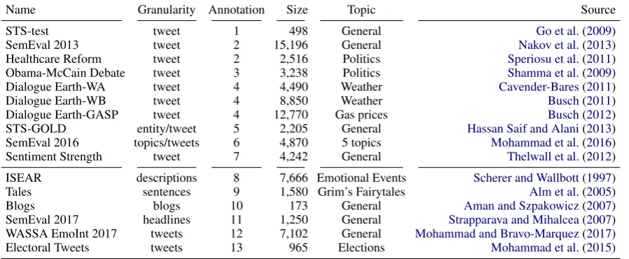
Table 1: A selection of resources for sentiment analysis (on Twitter, 1–7) and emotion analysis (in general, 8–12). Annotation refers to the following annotation schemes: [1] negative, [2] positive-negative-neutral, [3] positive-negative-mixed-other, [4] positive-negative-netural-unrelated-can’t tell, [5] positive-negative-neutral-mixed-other, [6] for-against, [7] positive and negative strength (range), [8] joy, fear, anger, sadness, disgust, shame, guilt, [9] angry, disgusted, fearful, happy, sad, positively surprised, negatively surprised, [10] happiness, sadness, anger, disgust, surprise, fear, mixed, [11] anger, disgust, fear, joy, sadness, surprise, [12] anger, fear, joy, sadness, [13] positive, negative, mixed, intensity, trust, fear, surprise, disgust, anger, anticipation, joy, roles, style, purpose (number denotes subset in corpus with emotion annotations)

For sentiment analysis, a large number of anno-tated data sets exists. These include review texts from different domains, for instance from Amazon and other shopping sites (Hu and Liu,2004;Ding et al.,2008;Toprak et al.,2010;Lakkaraju et al.,

2011), restaurants (Ganu et al.,2009), news articles (Wiebe et al.,2005), blogs (Kessler et al.,2010), as well as microposts on Twitter. For the latter, shown in the upper half of Table1, there are gen-eral corpora (Nakov et al.,2013;Spina et al.,2012;

Thelwall et al.,2012) as well as ones focused on very specific subdomains, for instance on Obama-McCain Debates (Shamma et al., 2009), Health Care Reforms (Speriosu et al.,2011). A popular example for a manually annotated corpus for senti-ment, which includes stance annotation for a set of topics is the SemEval 2016 data set (Mohammad et al.,2016).

For emotion analysis, the set of annotated re-sources is smaller (compare the lower half of Ta-ble 1). A very early resource is the ISEAR data set (Scherer and Wallbott, 1997) which contains descriptions of emotional events. While motivated by psychological research, it was later repurposed for computational research. The first data set devel-oped specifically for computational research was the tales corpus byAlm et al.(2005).Aman and

Sz-pakowicz(2007) published a corpus of blog posts. In the context of SemEval,Strapparava and Mihal-cea(2007) annotated news headlines.

A notable gap is the unavailability of a publicly available set of microposts (e. g., tweets) with emo-tion labels. To the best of our knowledge, there are only three previous approaches to labeling tweets with discrete emotion labels. One is the recent data set on for emotion intensity estimation, a shared task aiming at the development of a regression model. The goal is not to predict the emotion class, but a distribution over their intensities, and the set of emotions is limited tofear,sadness,anger, and joy(Mohammad and Bravo-Marquez,2017).

Label count for thresholdt

Emotion 0.0 0.33 0.5 0.66 0.99 Anger 2,902 2,238 1,388 1,315 578 Anticipation 2,700 1,656 739 677 199 Disgust 2,183 1,199 440 404 106 Fear 1,840 895 274 246 68 Joy 2,067 1,384 815 764 402 Sadness 2,644 1,389 414 343 78 Surprise 1,108 489 177 156 33 Trust 1,713 984 520 487 213

Table 2: Corpus Statistics. The threshold t mea-sures that a fraction of more thantannotators la-beled the respective emotion (e. g.,t=0.0: at least one annotatort=0.99: all annotators). Overall num-ber of tweets: 4,868.

Mohammad et al. (2015) annotated electoral tweets for sentiment, intensity, semantic roles, style, purpose and emotions. This is the only avail-able corpus similar to our work we are aware of. However, the focus of this work was not emotion annotation in contrast to ours. In addition, we pub-lish the data of all annotators.

3 Corpus Annotation and Analysis

3.1 Annotation Procedure

As motivated above, we re-annotate the extended SemEval 2016 Stance Data set (Mohammad et al.,

2016) which consists of 4,870 tweets (a subset of which was used in the SemEval competition). For a discussion of the differences of these data sets, we refer toMohammad et al.(2017). We omit two tweets with special characters, which leads to an overall set of 4,868 tweets used in our corpus.1

We frame annotation as a multi-label classifi-cation task at the tweet level. The tweets were annotated by a group of six independent annotators, with a minimum number of three annotations for each tweet (696 tweets were labeled by 6 annota-tors, 703 by 5 annotaannota-tors, 2,776 by 4 annotators and 693 by 3 annotators). All annotators were under-graduate students of media computer science and between the age of 20 and 30. Only one annotator is female. All students are German native speak-1_{Our annotations and original tweets are available}

at http://www.ims.uni-stuttgart.de/data/

ssec and http://alt.qcri.org/semeval2016/

task6/data/uploads/stancedataset.zip, see

alsohttp://alt.qcri.org/semeval2016/task6.

Cohen’sκ

Emotion Min Max

Anger 0.28 0.49

Anticipation 0.11 0.39 Disgust 0.06 0.30

Fear 0.08 0.25

Joy 0.30 0.52

Sadness 0.04 0.30 Surprise 0.09 0.33

Trust 0.29 0.57

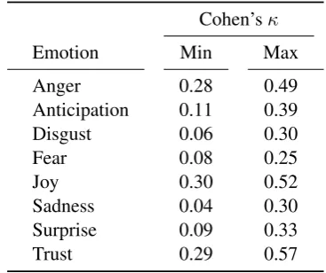
Table 3: Kappa Statistics for all pairs of annotators.

ers and have college-level proficiency in English. To train the annotators on the task, we performed two training iterations based on 50 randomly se-lected tweets from the SemEval 2016 Task 4 cor-pus (Nakov et al.,2016). After each iteration, we discussed annotation differences (informally) in face-to-face meetings.

For the final annotation, tweets were presented to the annotators in a web interface which paired a tweet with a set of binary check boxes, one for each emotion. Taggers could annotate any set of emotions. Each annotator was assigned with 5/7 of the corpus with equally-sized overlap of instances based on an offset shift. Not all annotators finished their task.2

3.2 Emotion Annotation Reliability and Aggregated Annotation

Our annotation represents a middle ground be-tween traditional linguistic “expert” annotation and crowdsourcing: We assume that intuitions about emotions diverge more than for linguistic structures. At the same time, we feel that there is information in the individual annotations beyond the simple “majority vote” computed by most crowdsourcing studies. In this section, we analyse the annotations intrinsically; a modelling-based evaluation follows in Section5.

Emotions Sentiment Stance

Anger Anticipation Disgust Fear Joy Sadness Surprise Trust Positi

ve

Ne

gati

ve

Neutral InFa

vor

Ag

ainst

None

Emotion

Anger 2902 1437 1983 1339 774 2065 711 640 275 2534 93 630 1628 644 Anticipation 0.55 2700 1016 1029 1330 1369 482 1234 1094 1445 161 772 1291 637 Disgust 19.05 0.52 2183 1024 512 1628 526 404 126 2008 49 429 1291 463 Fear 2.51 1.03 2.02 1840 466 1445 407 497 306 1445 89 448 982 410 Joy 0.19 1.88 0.22 0.30 2067 682 438 1101 1206 750 111 596 952 519 Sadness 5.91 0.72 4.82 5.58 0.21 2644 664 613 345 2171 128 604 1429 611 Surprise 1.28 0.54 1.15 0.94 0.86 1.34 1108 222 219 801 88 257 521 330 Trust 0.24 2.97 0.24 0.55 4.08 0.31 0.38 1713 1082 558 73 500 860 353

Sent.

Positive 0.06 2.75 0.06 0.30 10.94 0.13 0.46 10.53 1524 0 0 485 673 366 Negative 20.3 0.42 18.61 3.32 0.13 7.27 1.79 0.13 0.0 3032 0 622 1665 745 Neutral 0.26 0.85 0.21 0.64 0.73 0.56 1.36 0.54 0.0 0.0 312 97 71 144

Stance

In Favor 0.67 1.61 0.60 0.97 1.46 0.80 0.90 1.44 1.70 0.56 1.41 1204 0 0 Against 1.94 0.86 2.03 1.28 0.79 1.49 0.88 1.05 0.73 1.79 0.28 0.0 2409 0 None 0.63 0.77 0.64 0.74 0.94 0.74 1.30 0.65 0.87 0.85 2.66 0.0 0.0 1255

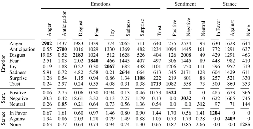
Table 4: Tweet Counts (above diagonal) and odds ratio (below diagonal) for cooccurring annotations for all classes in the corpus (emotions based on aggregated annotation,t=0.0).

precisionannotation. The other levels represent intermediate precision-recall trade-offs.

These numbers confirm that emotion labeling is a somewhat subjective task: only a small subset of the emotions labeled by at least one annotator (t=0.0) is labeled by most (t=0.66) or all of them (t=0.99). Interestingly, the exact percentage varies substantially by emotion, between 2 % forsadness and 20 % foranger.

Many of these disagreements stem from tweets that are genuinely difficult to categorize emotion-ally, like

That moment when Canadians realised global warming doesn’t equal a tropical vacation

for which one annotator choseangerandsadness, while one annotator chose surprise. Arguably, both annotations capture aspects of the meaning. Simi-larly, the tweet

2 pretty sisters are dancing with cancered kid

(a reference to an online video) is marked asfear and sadness by one annotator and with joy and sadnessby another. Naturally, not all differences arise from justified annotations. For instance the tweet

#BIBLE = Big Irrelevant Book of Lies and Exaggerations

has been labeled by two annotators with the emo-tiontrust, presumably because of the wordbible. This appears to be a classical oversight error, where the tweet is labeled on the basis of the first spotted keyword, without substantially studying its content.

To quantify these observations, we follow gen-eral practice and compute a chance-corrected mea-sure of inter-annotator agreement. Table3shows the minimum and maximum Cohen’sκvalues for pairs of annotators, computed on the intersection of instances annotated by either annotator within each pair. We obtain relatively highκ values of anger,joy, andtrust, but lower values for the other emotions.

These smallκvalues could be interpreted as in-dicators of problems with reliability. However,κis notoriously difficult to interpret, and a number of studies have pointed out the influence of marginal frequencies (Cicchetti and Feinstein,1990): In the presence of skewed marginals (and most of our emotion labels are quite rare,cf. Table2), the ex-pected agreement (referred to asP(E)in contrast toP(A)for the empirical agreement) is quite high. This makes it hard to obtain highκ values; thus, lowκvalues do not necessarily indicate unreliable annotation.

Emotions Sentiment Stance

Anger Anticipation Disgust Fear Joy Sadness Surprise Trust Positi

ve

Ne

gati

ve

Neutral InFa

vor

Ag

ainst

None

Emotion

Anger 1388 53 334 87 37 195 63 12 28 1353 7 272 840 276

Anticipation 0.16 739 16 42 218 14 2 182 445 253 41 258 333 148

Disgust 10.09 0.19 440 39 11 72 26 2 1 439 0 67 289 84

Fear 1.18 1.01 1.74 274 4 58 9 13 26 241 7 83 116 75

Joy 0.10 2.48 0.12 0.07 815 7 9 196 658 142 15 263 304 248

Sadness 2.43 0.18 2.34 3.20 0.08 414 14 3 28 377 9 102 216 96

Surprise 1.40 0.06 1.78 0.89 0.26 0.92 177 0 16 145 16 46 76 55 Trust 0.05 3.66 0.03 0.40 3.64 0.06 0.0 520 462 43 15 142 337 41

Sent.

Positive 0.03 4.28 0.0 0.22 15.42 0.14 0.21 24.65 1524 0 0 485 673 366 Negative 41.47 0.25 310.67 4.72 0.08 6.90 2.83 0.04 0.0 3032 0 622 1665 745 Neutral 0.05 0.84 0.0 0.37 0.24 0.30 1.48 0.41 0.0 0.0 312 97 71 144

Stance

In Favor 0.67 1.80 0.52 1.35 1.58 0.99 1.07 1.16 1.70 0.56 1.41 1204 0 0 Against 1.87 0.81 2.08 0.74 0.55 1.12 0.76 2.02 0.73 1.79 0.28 0.0 2409 0 None 0.63 0.68 0.66 1.09 1.32 0.86 1.31 0.22 0.87 0.85 2.66 0.0 0.0 1255

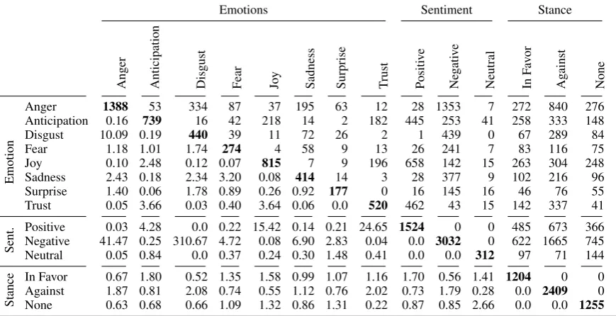
Table 5: Tweet Counts (above diagonal) and odds ratio (below diagonal) for cooccurring annotations for all classes in the corpus (emotions based on majority annotation,t=0.5).

high-recall annotation (see Section5 for details). We therefore define t=0.0 as ouraggregated an-notation. For comparison, we also considert=0.5, which corresponds to themajority annotation as generally adopted in crowdsourcing studies.

3.3 Distribution of Emotions

As shown in Table2, nearly 60 % of the overall tweet set are annotated withangerby at least one annotator. This is the predominant emotion class, followed byanticipationandsadness. This distribu-tion is comparably uncommon and originates from the selection of tweets in SemEval as a stance data set. However, whileanger clearly dominates in the aggregated annotation, its predominance weak-ens for the more precision-oriented data sets. For

t=0.99,joybecomes the second most frequent emo-tion. In uniform samples from Twitter, joy typically dominates the distribution of emotions (Klinger,

2017). It remains a question for future work how to reconciliate these observations.

3.4 Emotion vs. other Annotation Layers Table 4 shows the number of cooccurring label pairs (above the diagonal) and the odds ratios (be-low the diagonal) for emotion, stance, and sen-timent annotations on the whole corpus for our aggregated annotation (t=0.0). Odds ratio is

R(A:B)= P_P(₍A_B)(1₎₍₁−₋P_P(₍B_A))₎₎,

whereP(A)is the probability that both labels (at row and column in the table) hold for a tweet and

P(B) is the probability that only one holds. A ratio ofxmeans that the joint labeling isxtimes more likely than the independent labeling. Table5

shows the same numbers for the majority annota-tion,t=0.5.

We first analyze the relationship between emo-tions and sentiment polarity in Table4. For many emotions, the polarity is as expected:Joyandtrust occur predominantly with positive sentiment, and anger, disgust,fearandsadnesswith negative sen-timent. The emotionsanticipationandsurpriseare, in comparison, most balanced between polarities, however with a majority for positive sentiment in anticipation and a negative sentiment for surprise. For most emotions there is also a non-negligible number of tweets with the sentiment opposite to a common expectation. For example,angeroccurs 28 times with positive sentiment, mainly tweets which call for (positive) change regarding a contro-versial topic, for instance

Lets take back our country! Whos with me? No more Democrats!2016

Why criticise religions? If a path is not your own. Don’t be pretentious. And get down from your throne.

either the emotion annotator or the sentiment an-notator assumed some non-literal meaning to be associated with the text (mainly irony), for instance

Global Warming! Global Warming! Global Warming! Oh wait, it’s summer. I love the smell of Hillary in the morning. It smells like Republican Victory.

Disgust occurs almost exclusively with negative sentiment.

For the majority annotation (Table5), the num-ber of annotations is smaller. However, the average size of the odds ratios increase (from 1.96 fort=0.0 to 5.39 fort=0.5).

A drastic example isdisgustin combination with negative sentiment, the predominant combination. Disgustis only labeled once with positive sentiment in thet=0.5 annotation:

#WeNeedFeminism because #NoMeansNo it doesnt mean yes, it doesnt mean try harder!

Similarly, the odds ratio for the combinationanger and negative sentiment nearly doubles from 20.3 fort=0.0 to 41.47 fort=0.5. These numbers are an effect of the majority annotation having a higher precision in contrast to more “noisy” aggregation of all annotations (t=0.0).

Regarding the relationship between emotions and stance, most odds ratios are relatively close to 1, indicating the absence of very strong correlations. Nevertheless, the ”Against” stance is associated with a number of negative emotions (anger, disgust, sadness, the ”In Favor” stance withjoy, trust,and anticipation, and ”None” with an absence of all emotions exceptsurprise.

4 Models

We apply six standard models to provide base-line results for our corpus: Maximum Entropy (MAXENT), Support Vector Machines (SVM), a

Long-Short Term Memory Network (LSTM), a Bidirectional LSTM (BI-LSTM), and a

Convolu-tional Neural Network (CNN).

MaxEnt and SVM classify each tweet sepa-rately based on a bag-of-words. For the first, the lin-ear separator is estimated based on log-likelihood optimization with an L2 prior. For the second, the optimization follows a max-margin strategy.

LSTM(Hochreiter and Schmidhuber,1997) is a recurrent neural network architecture which in-cludes a memory state capable of learning long distance dependencies. In various forms, they have proven useful for text classification tasks (Tai et al.,

2015;Tang et al.,2016). We implement a standard LSTM which has an embedding layer that maps the input (padded when needed) to a 300 dimensional vector. These vectors then pass to a 175 dimen-sional LSTM layer. We feed the final hidden state to a fully-connected 50-dimensional dense layer and use sigmoid to gate our 8 output neurons. As a regularizer, we use a dropout (Srivastava et al.,

2014) of 0.5 before the LSTM layer.

Bi-LSTMhas the same architecture as the nor-mal LSTM, but includes an additional layer with a reverse direction. This approach has produced state-of-the-art results for POS-tagging (Plank et al.,

2016), dependency parsing (Kiperwasser and Gold-berg, 2016) and text classification (Zhou et al.,

2016), among others. We use the same parame-ters as the LSTM, but concatenate the two hidden layers before passing them to the dense layer.

CNN has proven remarkably effective for text classification (Kim, 2014;dos Santos and Gatti,

2014; Flekova and Gurevych, 2016) . We train a simple one-layer CNN with one convolutional layer on top of pre-trained word embeddings, fol-lowingKim(2014). The first layer is an embed-dings layer that maps the input of lengthn(padded when needed) to an n x 300 dimensional matrix. The embedding matrix is then convoluted with fil-ter sizes of 2, 3, and 4, followed by a pooling layer of length 2. This is then fed to a fully connected dense layer with ReLu activations and finally to the 8 output neurons, which are gated with the sigmoid function. We again use dropout (0.5), this time before and after the convolutional layers.

For all neural models, we initialize our word rep-resentations with the skip-gram algorithm with neg-ative sampling (Mikolov et al.,2013), trained on nearly 8 million tokens taken from tweets collected using various hashtags. We create 300-dimensional vectors with window size 5, 15 negative samples and run 5 iterations. For OOV words, we use a vec-tor initialized randomly between -0.25 and 0.25 to approximate the variance of the pretrained vectors. We train our models using ADAM (Kingma and Ba,

Results for Thresholdt= 0.0for standard models

Linear Neural

MAXENT SVM LSTM Bi-LSTM CNN

Emotion P R F1 P R F1 P R F1 P R F1 P R F1

Anger 76 72 74 76 69 72 76

(1.7) (5.3)77 (1.9)76 (0.8)77 (2.7)77 (1.3)77 (0.8)77 (2.7)77 (1.3)77 Anticipation 72 61 66 70 60 64 68

(1.8) (8.9)68 (3.5)67 (1.2)70 (3.6)66 (1.6)68 (1.2)68 (0.8)60 (0.5)64

Disgust 62 47 54 59 53 56 64

(3.2) (8.7)68 (2.5)65 (1.4)61 (4.6)64 (1.7)63 (0.6)62 (3.9)61 (1.9)62

Fear 57 31 40 55 40 46 51

(3.5) (8.5)48 (4.6)49 (1.6)58 (6.3)43 (3.8)49 (1.7)53 (6.2)46 (3.9)49

Joy 55 50 52 52 52 52 56

(5.9) (8.3)41 (4.8)46 (2.9)54 (10.5)59 (4.8)56 (1.7)54 (5.6)56 (2.3)55

Sadness 65 65 65 64 60 62 60

(2.5) (11.1)77 (3.9)67 (0.6)62 (7.5)72 (3.2)67 (0.9)63 (0.3)72 (0.5)67

Surprise 62 15 24 46 22 30 40

(4.4) (10.4)17 (8.7)21 (2.9)42 (3.2)20 (2.5)27 (3.7)36 (6.3)24 (5.0)28

Trust 62 38 47 57 45 50 57

(6.1) (12.3)49 (5.9)51 (2.5)59 (4.1)44 (2.5)50 (0.6)53 (6.6)49 (3.3)50

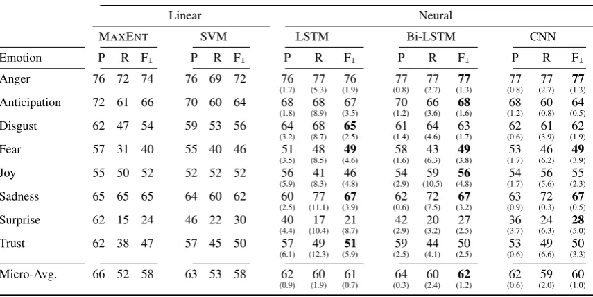
Micro-Avg. 66 52 58 63 53 58 62

(0.9) (1.9)60 (0.7)61 (0.3)64 (2.4)60 (1.2)62 (0.6)62 (2.0)59 (1.0)60 Table 6: Results of linear and neural models for labels from the aggregated annotation (t=0.0). For the neural models, we report the average of five runs and standard deviation in brackets. Best F1 for each

emotion shown in boldface.

the training data aside to tune the hyperparameters for each model (hidden dimension size, dropout rate, and number of training epochs).

5 Results

Table6shows the results for our canonical annota-tion aggregaannota-tion witht=0.0 (aggregated annotation) for our models. The two linear classifiers (trained as MAXENTand SVM) show comparable results,

with an overall micro-average F1of 58 %. All

neu-ral network approaches show a higher performance of at least 2 percentage points (3 pp for LSTM, 4 pp for BI-LSTM, 2 pp for CNN). BI-LSTM also

ob-tains the best F-Score for 5 of the 8 emotions (4 out of 8 for LSTM and CNN). We conclude that the BI-LSTM shows the best results of all our models.

Our discussion focuses on this model.

The performance clearly differs between emo-tion classes. Recall from Secemo-tion3.2thatanger, joy andtrustshowed much higher agreement numbers than the other annotations. There is however just a mild correlation between reliability and model-ing performance. Angeris indeed modelled very well: it shows the best prediction performance with a similar precision and recall on all models. We ascribe this to it being the most frequent emotion class. In contrast,joyandtrustshow only middling performance, while we see relatively good results foranticipationandsadnesseven though there was considerable disagreement between annotators. We

find the overall worst results forsurprise. This is not surprising,surprisebeing a scarce label with also very low agreement. This might point towards underlying problems in the definition ofsurprise as an emotion. Some authors have split this class into positive and negative surprise in an attempt to avoid this (Alm et al.,2005).

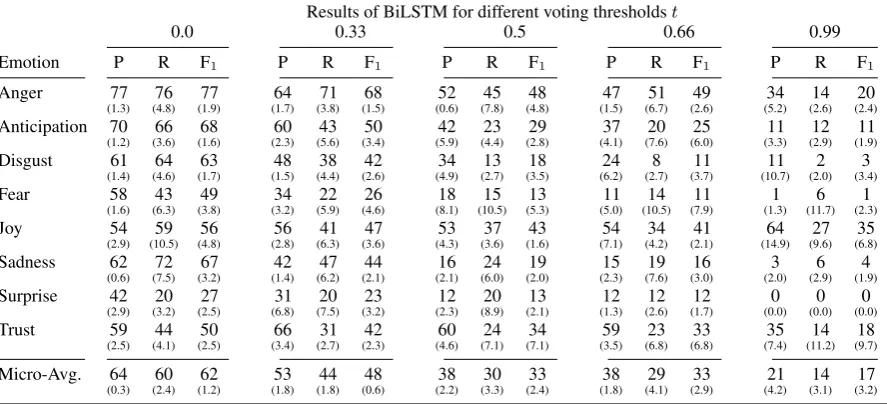
We finally come to our justification for choos-ing t=0.0 as our aggregated annotation. Table7

shows results for the best model (BI-LSTM) on

the datasets for different thresholds. We see a clear downward monotone trend: The higher the thresh-old, the lower the F1 measures. We obtain the

Results of BiLSTM for different voting thresholdst

0.0 0.33 0.5 0.66 0.99

Emotion P R F1 P R F1 P R F1 P R F1 P R F1

Anger 77

(1.3) (4.8)76 (1.9)77 (1.7)64 (3.8)71 (1.5)68 (0.6)52 (7.8)45 (4.8)48 (1.5)47 (6.7)51 (2.6)49 (5.2)34 (2.6)14 (2.4)20 Anticipation 70

(1.2) (3.6)66 (1.6)68 (2.3)60 (5.6)43 (3.4)50 (5.9)42 (4.4)23 (2.8)29 (4.1)37 (7.6)20 (6.0)25 (3.3)11 (2.9)12 (1.9)11 Disgust 61

(1.4) (4.6)64 (1.7)63 (1.5)48 (4.4)38 (2.6)42 (4.9)34 (2.7)13 (3.5)18 (6.2)24 (2.7)8 (3.7)11 (10.7)11 (2.0)2 (3.4)3

Fear 58

(1.6) (6.3)43 (3.8)49 (3.2)34 (5.9)22 (4.6)26 (8.1)18 (10.5)15 (5.3)13 (5.0)11 (10.5)14 (7.9)11 (1.3)1 (11.7)6 (2.3)1

Joy 54

(2.9) (10.5)59 (4.8)56 (2.8)56 (6.3)41 (3.6)47 (4.3)53 (3.6)37 (1.6)43 (7.1)54 (4.2)34 (2.1)41 (14.9)64 (9.6)27 (6.8)35 Sadness 62

(0.6) (7.5)72 (3.2)67 (1.4)42 (6.2)47 (2.1)44 (2.1)16 (6.0)24 (2.0)19 (2.3)15 (7.6)19 (3.0)16 (2.0)3 (2.9)6 (1.9)4 Surprise 42

(2.9) (3.2)20 (2.5)27 (6.8)31 (7.5)20 (3.2)23 (2.3)12 (8.9)20 (2.1)13 (1.3)12 (2.6)12 (1.7)12 (0.0)0 (0.0)0 (0.0)0

Trust 59

(2.5) (4.1)44 (2.5)50 (3.4)66 (2.7)31 (2.3)42 (4.6)60 (7.1)24 (7.1)34 (3.5)59 (6.8)23 (6.8)33 (7.4)35 (11.2)14 (9.7)18 Micro-Avg. 64

(0.3) (2.4)60 (1.2)62 (1.8)53 (1.8)44 (0.6)48 (2.2)38 (3.3)30 (2.4)33 (1.8)38 (4.1)29 (2.9)33 (4.2)21 (3.1)14 (3.2)17 Table 7: Results of the BiLSTM for different voting thresholds. We report average results for each emotion over 5 runs (standard deviations are included in parenthesis).

most useful datasets from a computational model-ing perspective.

In terms of how to deal with diverging annota-tions, we believe that this result bolsters our general approach to pay attention to individual annotators’ labels rather than just majority votes: if the individ-ual labels were predominantly noisy, we would not expect to see relatively high F1scores.

6 Conclusion and Future Work

With this paper, we publish the first manual emo-tion annotaemo-tion for a publicly available micropost corpus. The resource we chose to annotate already provides stance and sentiment information. We an-alyzed the relationships among emotion classes and between emotions and the other annotation layers. In addition to the data set, we implemented well-known standard models which are established for sentiment and polarity prediction for emotion clas-sification. The BI-LSTM model outperforms all

other approaches by up to 4 points F1on average

compared to linear classifiers.

Inter-annotator analysis showed a limited agree-ment between the annotators – the task is, at least to some degree, driven by subjective opinions. We found, however, that this is not necessarily a prob-lem: Our models perform best on a high-recall aggregate annotationwhich includes all labels as-signed by at least one annotator. Thus, we believe that the individual labels have value and are not, like generally assumed in crowdsourcing, noisy inputs suitable only as input for majority voting.

In this vein, we publish all individual annotations. This enables further research on other methods of defining consensus annotations which may be more appropriate for specific downstream tasks. More generally, we will make all annotations, resources and model implementations publicly available.

References

Cecilia Ovesdotter Alm, Dan Roth, and Richard Sproat. 2005. Emotions from text: Machine learning for text-based emotion prediction. InProceedings of Human Language Technology Conference and Conference on Empirical Methods in Natural Lan-guage Processing, pages 579–586, Vancouver, BC, Canada.

Saima Aman and Stan Szpakowicz. 2007. Identifying expressions of emotion in text. InText, Speech and Dialogue: 10th International Conference, TSD 2007, Pilsen, Czech Republic, September 3-7, 2007. Pro-ceedings, pages 196–205. Springer.

Isabelle Augenstein, Andreas Vlachos, and Kalina Bontcheva. 2016. USFD at semeval-2016 task 6: Any-target stance detection on twitter with autoen-coders. In Proceedings of the 10th International Workshop on Semantic Evaluation (SemEval-2016), pages 389–393, San Diego, California.

Sarah Busch. 2011. Capturing mood

about daily weather from twitter posts. http://www.dialogueearth.org/2011/09/29/capturing-mood-about-daily-weather-from-twitter-posts. Sarah Busch. 2012. Tracking the mood

Kent Cavender-Bares. 2011. Preparing to extract weather mood from tweets. http://www.dialogueearth.org/2011/03/03/preparing-to-extract-weather-mood-from-tweets.

Domenic V. Cicchetti and Alvan R. Feinstein. 1990. High agreement but low kappa: II. resolving the paradoxes. Journal of clinical epidemiology, 43:551–558.

Joana Costa, Catarina Silva, Mario Antunes, and Bernardete Ribeiro. 2014. Concept drift awareness in twitter streams. In13th International Conference on Machine Learning and Applications, pages 294– 299.

Marcelo Dias and Karin Becker. 2016. INF-UFRGS-OPINION-MINING at SemEval-2016 task 6: Au-tomatic generation of a training corpus for unsuper-vised identification of stance in tweets. In Proceed-ings of the 10th International Workshop on Seman-tic Evaluation (SemEval-2016), pages 378–383, San Diego, California.

Xiaowen Ding, Bing Liu, and Philip S. Yu. 2008. A holistic lexicon-based approach to opinion mining. InWSDM ’08 Proceedings of the 2008 International Conference on Web Search and Data Mining, pages 213–239, Palo Alto, California, USA.

Peter S. Dodds, Kameron D. Harris, Isabel M. Kloumann, Catherine A. Bliss, and Christopher M. Danforth. 2011. Temporal patterns of happiness and information in a global social network: Hedonomet-rics and twitter.PloS one, 6(12).

Javid Ebrahimi, Dejing Dou, and Daniel Lowd. 2016. Weakly supervised tweet stance classification by re-lational bootstrapping. In Proceedings of the 2016 Conference on Empirical Methods in Natural Lan-guage Processing, pages 1012–1017, Austin, Texas. Paul Ekman. 1999. Basic emotions. In M Dalgleish, T; Power, editor,Handbook of Cognition and Emo-tion. John Wiley & Sons, Sussex, UK.

Lucie Flekova and Iryna Gurevych. 2016. Supersense embeddings: A unified model for supersense inter-pretation, prediction, and utilization. InProceedings of the 54th Annual Meeting of the Association for Computational Linguistics (Volume 1: Long Papers), pages 2029–2041, Berlin, Germany.

Gayatree Ganu, Noemie Elhadad, and Am´elie Marian. 2009. Beyond the stars: Improving rating predic-tions using review text content. In International Workshop on the Web and Databases (WebDB 2009), Providence, Rhode Island, USA.

Alec Go, Richa Bhayani, and Lei Huang. 2009. Twit-ter sentiment classification using distant supervision. Technical report, Stanford.

Yulan He Hassan Saif, Miriam Fernandez and Harith Alani. 2013. Evaluation Datasets for Twitter Sen-timent Analysis: A survey and a new dataset, the

STS-Gold. In Proceedings of the First Interna-tional Workshop on Emotion and Sentiment in Social and Expressive Media: approaches and perspectives from AI (ESSEM 2013), pages 9–21, Turin, Italy. Sepp Hochreiter and J¨urgen Schmidhuber. 1997.

Long short-term memory. Neural Computation, 9(8):1735–1780.

Minqing Hu and Bing Liu. 2004. Mining and sum-marizing customer reviews. InKDD ’04 Proceed-ings of the tenth ACM SIGKDD international con-ference on Knowledge discovery and data mining, pages 168–177, Seattle, WA, USA.

Jason S. Kessler, Miriam Eckert, Lyndsie Clark, and Nicolas Nicolov. 2010. The 2010 ICWSM JDPA Sentiment Corpus for the Automotive Domain. In Proc. of the 4th International AAAI Conference on Weblogs and Social Media Data Workshop Chal-lenge (ICWSM-DWC).

Yoon Kim. 2014. Convolutional neural networks for sentence classification. In Proceedings of the 2014 Conference on Empirical Methods in Natural Language Processing (EMNLP), pages 1746–1751, Doha, Qatar.

Diederik Kingma and Jimmy Ba. 2015. Adam: A method for stochastic optimization. InProceedings of International Conference on Learning Represen-tations, San Diego, CA, USA.

Eliyahu Kiperwasser and Yoav Goldberg. 2016. Sim-ple and accurate dependency parsing using bidirec-tional LSTM feature representations. Transactions of the Association for Computational Linguistics, 4:313–327.

Roman Klinger. 2017. Does optical character recog-nition and caption generation improve emotion de-tection in microblog posts? InNatural Language Processing and Information Systems: 22nd Interna-tional Conference on Applications of Natural Lan-guage to Information Systems, NLDB 2017, Li`ege, Belgium, June 21-23, 2017, Proceedings, pages 313– 319, Cham. Springer International Publishing. Himabindu Lakkaraju, Chiranjib Bhattacharyya,

Indra-jit Bhattacharya, and Srujana Merugu. 2011. Ex-ploiting coherence for the simultaneous discovery of latent facets and associated sentiments. In Proceed-ings of the 2011 SIAM International Conference on Data Mining, pages 498–509, Mesa, Arizona, USA. Tomas Mikolov, Greg Corrado, Kai Chen, and Jeffrey Dean. 2013. Efficient estimation of word represen-tations in vector space. In Proceedings of Inter-national Conference on Learning Representations, Scottsdale, AZ, USA.

Saif Mohammad, Svetlana Kiritchenko, Parinaz Sob-hani, Xiaodan Zhu, and Colin Cherry. 2016. SemEval-2016 Task 6: Detecting stance in tweets. In Proceedings of the 10th International Workshop on Semantic Evaluation (SemEval-2016), pages 31– 41, San Diego, California.

Saif M. Mohammad, Parinaz Sobhani, and Svetlana Kiritchenko. 2017. Stance and sentiment in tweets. Special Section of the ACM Transactions on Inter-net Technology on Argumentation in Social Media, 17(3).

Saif M. Mohammad, Xiaodan Zhu, Svetlana Kir-itchenko, and Joel Martin. 2015. Sentiment, emo-tion, purpose, and style in electoral tweets. Informa-tion Processing & Management, 51(4):480 – 499.

Myriam Munezero, Calkin Suero Montero, Erkki Su-tinen, and John Pajunen. 2014. Are they different? Affect, feeling, emotion, sentiment, and opinion de-tection in text. IEEE Transactions on Affective Com-puting, 5(2):101–111.

Preslav Nakov, Alan Ritter, Sara Rosenthal, Veselin Stoyanov, and Fabrizio Sebastiani. 2016. SemEval-2016 task 4: Sentiment analysis in Twitter. In Pro-ceedings of the 10th International Workshop on Se-mantic Evaluation, SemEval ’16, San Diego, Cali-fornia. Association for Computational Linguistics.

Preslav Nakov, Sara Rosenthal, Zornitsa Kozareva, Veselin Stoyanov, Alan Ritter, and Theresa Wilson. 2013. SemEval-2013 Task 2: Sentiment analysis in twitter. InSecond Joint Conference on Lexical and Computational Semantics (*SEM), Volume 2: Pro-ceedings of the Seventh International Workshop on Semantic Evaluation (SemEval 2013), pages 312– 320, Atlanta, Georgia, USA.

Barbara Plank, Anders Søgaard, and Yoav Goldberg. 2016. Multilingual part-of-speech tagging with bidi-rectional long short-term memory models and auxil-iary loss. InProceedings of the 54th Annual Meet-ing of the Association for Computational LMeet-inguistics (Volume 2: Short Papers), pages 412–418, Berlin, Germany.

Robert Plutchik. 2001. The nature of emotions. Ameri-can Scientist, 89(July–August):344–350.

Matthew Purver and Stuart Battersby. 2012. Experi-menting with distant supervision for emotion classi-fication. In Proceedings of the 13th Conference of the European Chapter of the Association for Com-putational Linguistics, pages 482–491, Avignon, France.

Kirk Roberts, Michael A. Roach, Joseph Johnson, Josh Guthrie, and Sanda M. Harabagiu. 2012. Em-patweet: Annotating and detecting emotions on twit-ter. In Proceedings of the Eighth International Conference on Language Resources and Evaluation (LREC-2012), pages 3806–3813, Istanbul, Turkey.

Cicero dos Santos and Maira Gatti. 2014. Deep con-volutional neural networks for sentiment analysis of short texts. In Proceedings of COLING 2014, the 25th International Conference on Computational Linguistics: Technical Papers, pages 69–78, Dublin, Ireland.

Klaus Scherer and Harald Wallbott. 1997. The ISEAR questionnaire and codebook. Geneva Emotion Re-search Group.

David A. Shamma, Lyndon Kennedy, and Elizabeth F. Churchill. 2009. Tweet the debates: Understanding community annotation of uncollected sources. In Proceedings of the First SIGMM Workshop on So-cial Media, pages 3–10, Beijing, China.

Michael Speriosu, Nikita Sudan, Sid Upadhyay, and Ja-son Baldridge. 2011. Twitter polarity classification with label propagation over lexical links and the fol-lower graph. InProceedings of the First workshop on Unsupervised Learning in NLP, pages 53–63, Ed-inburgh, Scotland.

Damiano Spina, Edgar Meij, Maarten de Rijke, An-drei Oghina, Minh Thuong Bui, and Mathias Breuss. 2012. Identifying entity aspects in microblog posts. InProceedings of the 35th International ACM SIGIR Conference on Research and Development in Infor-mation Retrieval, pages 1089–1090, New York, NY, USA. ACM.

Nitish Srivastava, Geoffrey Hinton, Alex Krizhevsky, and Ruslan Salakhutdinov. 2014. Dropout: A sim-ple way to prevent neural networks from overfitting. Journal of Machine Learning Research, 15:1929– 1958.

Carlo Strapparava and Rada Mihalcea. 2007. SemEval-2007 Task 14: Affective Text. InProceedings of the Fourth International Workshop on Semantic Evalua-tions (SemEval-2007), pages 70–74, Prague, Czech Republic.

Jared Suttles and Nancy Ide. 2013. Distant supervision for emotion classification with discrete binary val-ues. In Computational Linguistics and Intelligent Text Processing: 14th International Conference, CI-CLing 2013, Samos, Greece, March 24-30, 2013, Proceedings, Part II, pages 121–136, Berlin, Heidel-berg. Springer Berlin HeidelHeidel-berg.

Kai Sheng Tai, Richard Socher, and Christopher D. Manning. 2015. Improved semantic representations from tree-structured long short-term memory net-works. In Proceedings of the 53rd Annual Meet-ing of the Association for Computational LMeet-inguistics and the 7th International Joint Conference on Natu-ral Language Processing (Volume 1: Long Papers), pages 1556–1566, Beijing, China.

2016, the 26th International Conference on Compu-tational Linguistics: Technical Papers, pages 3298– 3307, Osaka, Japan.

Mike Thelwall, Kevan Buckley, and Georgios Pal-toglou. 2012. Sentiment strength detection for the social web. Journal of the American Society for In-formation Science Technology, 63(1):163–173. Cigdem Toprak, Niklas Jakob, and Iryna Gurevych.

2010. Sentence and expression level annotation of opinions in user-generated discourse. In Proceed-ings of the 48th Annual Meeting of the Association for Computational Linguistics, pages 575–584, Up-psala, Sweden.

Wenbo Wang, Lu Chen, Krishnaprasad Thirunarayan, and Amit P. Sheth. 2012. Harnessing twitter ”big data” for automatic emotion identification. In2012 ASE/IEEE International Conference on Social Com-puting and 2012 ASE/IEEE International Confer-ence on Privacy, Security, Risk and Trust, pages 587–592, Washington, DC, USA.

Wan Wei, Xiao Zhang, Xuqin Liu, Wei Chen, and Tengjiao Wang. 2016. pkudblab at SemEval-2016 Task 6: A specific convolutional neural network sys-tem for effective stance detection. InProceedings of the 10th International Workshop on Semantic Eval-uation (SemEval-2016), pages 384–388, San Diego, California.

Janyce Wiebe, Theresa Wilson, and Claire Cardie. 2005. Annotating expressions of opinions and emo-tions in language. Language Resources and Evalua-tion, 39(2-3).