An Overview on Application of Machine Learning Techniques in Optical Networks

An Overview on Application of Machine Learning

Techniques in Optical Networks

Francesco Musumeci,

Member, IEEE,

Cristina Rottondi,

Member, IEEE,

Avishek Nag,

Member, IEEE,

Irene

Macaluso, Darko Zibar,

Member, IEEE,

Marco Ruffini,

Senior Member, IEEE,

and Massimo

Tornatore,

Senior Member, IEEE

Abstract—Today’s telecommunication networks have become sources of enormous amounts of widely heterogeneous data. This information can be retrieved from network traffic traces, network alarms, signal quality indicators, users’ behavioral data, etc. Advanced mathematical tools are required to extract meaningful information from these data and take decisions pertaining to the proper functioning of the networks from the network-generated data. Among these mathematical tools, Machine Learning (ML) is regarded as one of the most promising methodological ap-proaches to perform network-data analysis and enable automated network self-configuration and fault management.

The adoption of ML techniques in the field of optical com-munication networks is motivated by the unprecedented growth of network complexity faced by optical networks in the last few years. Such complexity increase is due to the introduction of a huge number of adjustable and interdependent system parameters (e.g., routing configurations, modulation format, symbol rate, coding schemes, etc.) that are enabled by the usage of coherent transmission/reception technologies, advanced digital signal processing and compensation of nonlinear effects in optical fiber propagation.

In this paper we provide an overview of the application of ML to optical communications and networking. We classify and survey relevant literature dealing with the topic, and we also provide an introductory tutorial on ML for researchers and practitioners interested in this field. Although a good number of research papers have recently appeared, the application of ML to optical networks is still in its infancy: to stimulate further work in this area, we conclude the paper proposing new possible research directions.

Index Terms—Machine learning, Data analytics, Optical com-munications and networking, Neural networks, Bit Error Rate, Optical Signal-to-Noise Ratio, Network monitoring.

I. INTRODUCTION

Machine learning (ML) is a branch of Artificial Intelligence that pushes forward the idea that, by giving access to the right data, machines can learn by themselves how to solve a specific problem [1]. By leveraging complex mathematical and statistical tools, ML renders machines capable of performing independently intellectual tasks that have been traditionally Francesco Musumeci and Massimo Tornatore are with Po-litecnico di Milano, Italy, e-mail: [email protected], [email protected]

Cristina Rottondi is with Dalle Molle Institute for Artificial Intelligence, Switzerland, email: [email protected].

Avishek Nag is with University College Dublin, Ireland, email: [email protected].

Irene Macaluso and Marco Ruffini are with Trinity College Dublin, Ireland, email: [email protected], [email protected].

Darko Zibar is with Technical University of Denmark, Denmark, email: [email protected].

solved by human beings. This idea of automating complex tasks has generated high interest in the networking field, on the expectation that several activities involved in the design and operation of communication networks can be offloaded to machines. Some applications of ML in different networking areas have already matched these expectations in areas such as intrusion detection [2], traffic classification [3], cognitive radios [4].

Among various networking areas, in this paper we focus on ML for optical networking. Optical networks constitute the basic physical infrastructure of all large-provider networks worldwide, thanks to their high capacity, low cost and many other attractive properties [5]. They are now penetrating new important telecom markets as datacom [6] and the access segment [7], and there is no sign that a substitute technology might appear in the foreseeable future. Different approaches to improve the performance of optical networks have been investigated, such as routing, wavelength assignment, traffic grooming and survivability [8], [9].

In this paper we give an overview of the application of ML to optical networking. Specifically, the contribution of the paper is twofold, namely, i) we provide an introductory tutorial on the use of ML methods and on their application in the optical networks field, andii) we survey the existing work dealing with the topic, also performing a classification of the various use cases addressed in literature so far. We cover both the areas of optical communication and optical networking to potentially stimulate new cross-layer research directions. In fact, ML application can be useful especially in cross-layer settings, where data analysis at physical layer, e.g., monitoring Bit Error Rate (BER), can trigger changes at network layer, e.g., in routing, spectrum and modulation format assignments. The application of ML to optical communication and network-ing is still in its infancy and the literature survey included in this paper aims at providing an introductory reference for researchers and practitioners willing to get acquainted with existing ML applications as well as to investigate new research directions.

in the complexity of optical networks.

On a system side, while optical channel modeling has always been complex, the recent adoption of coherent tech-nologies [11] has made modeling even more difficult by introducing a plethora of adjustable design parameters (as modulation formats, symbol rates, adaptive coding rates and flexible channel spacing) to optimize transmission systems in terms of bit-rate transmission distance product. In addition, what makes this optimization even more challenging is that the optical channel is highly nonlinear.

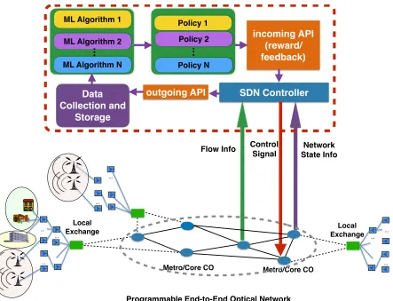
From a networking perspective, the increased complexity of the underlying transmission systems is reflected in a series of advancements in both data plane and control plane. At data plane, the Elastic Optical Network (EON) concept [12]–[15] has emerged as a novel optical network architecture able to respond to the increased need of elasticity in allocating optical network resources. In contrast to traditional fixed-grid Wave-length Division Multiplexing (WDM) networks, EON offers flexible (almost continuous) bandwidth allocation. Resource allocation in EON can be performed to adapt to the several above-mentioned decision variables made available by new transmission systems, including different transmission tech-niques, such as Orthogonal Frequency Division Multiplexing (OFDM), Nyquist WDM (NWDM), transponder types (e.g., BVT1_{, S-BVT), modulation formats (e.g., QPSK, QAM), and} coding rates. This flexibility makes the resource allocation problems much more challenging for network engineers. At control plane, dynamic control, as in Software-defined net-working (SDN), promises to enable long-awaited on-demand reconfiguration and virtualization. Moreover, reconfiguring the optical substrate poses several challenges in terms of, e.g., network re-optimization, spectrum fragmentation, amplifier power settings, unexpected penalties due to non-linearities, which call for strict integration between the control elements (SDN controllers, network orchestrators) and optical perfor-mance monitors working at the equipment level.

All these degrees of freedom and limitations do pose severe challenges to system and network engineers when it comes to deciding what the best system and/or network design is. Machine learning is currently perceived as a paradigm shift for the design of future optical networks and systems. These techniques should allow to infer, from data obtained by various types of monitors (e.g., signal quality, traffic samples, etc.), useful characteristics that could not be easily or directly measured. Some envisioned applications in the optical domain include fault prediction, intrusion detection, physical-flow security, impairment-aware routing, low-margin design, traffic-aware capacity reconfigurations, but many others can be envisioned and will be surveyed in the next sections.

The survey is organized as follows. In Section II, we overview some preliminary ML concepts, focusing especially on those targeted in the following sections. In Section III we discuss the main motivations behind the application of ML in the optical domain and we classify the main areas of applications. In Section IV and Section V, we classify and

1_{For a complete list of acronyms, the reader is referred to the Glossary at} the end of the paper.

summarize a large number of studies describing applications of ML at the transmission layer and network layer. In Section VI, we quantitatively overview a selection of existing papers, identifying, for some of the applications described in Section III, the ML algorithms which demonstrated higher effective-ness for each specific use case, and the performance metrics considered for the algorithms evaluation. Finally, Section VII discusses some possible open areas of research and future directions, whereas Section VIII concludes the paper.

II. OVERVIEW OF MACHINE LEARNING METHODS USED IN OPTICAL NETWORKS

This section provides an overview of some of the most popular algorithms that are commonly classified as machine learning. The literature on ML is so extensive that even a superficial overview of all the main ML approaches goes far beyond the possibilities of this section, and the readers can refer to a number of fundamental books on the subjects [16]– [20]. However, in this section we provide a high level view of the main ML techniques that are used in the work we reference in the remainder of this paper. We here provide the reader with some basic insights that might help better understand the remaining parts of this survey paper. We divide the algorithms in three main categories, described in the next sections, which are also represented in Fig. 1: supervised learning, unsuper-vised learning and reinforcement learning. Semi-superunsuper-vised learning, a hybrid of supervised and unsupervised learning, is also introduced. ML algorithms have been successfully applied to a wide variety of problems. Before delving into the different ML methods, it is worth pointing out that, in the context of telecommunication networks, there has been over a decade of research on the application of ML techniques to wireless networks, ranging from opportunistic spectrum access [21] to channel estimation and signal detection in OFDM systems [22], to Multiple-Input-Multiple-Output communications [23], and dynamic frequency reuse [24].

A. Supervised learning

Supervised learning is used in a variety of applications, such as speech recognition, spam detection and object recognition. The goal is to predict the value of one or more output variables given the value of a vector of input variables x. The output variable can be a continuous variable (regression problem) or a discrete variable (classification problem). A training data set comprises N samples of the input variables and the corresponding output values. Different learning methods construct a function y(x) that allows to predict the value of the output variables in correspondence to a new value of the inputs. Supervised learning can be broken down into two main classes, described below: parametric models, where the number of parameters to use in the model is fixed, and non-parametric models, where their number is dependent on the training set.

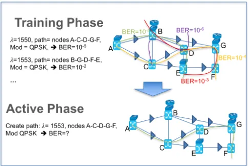
(a) Supervised Learning: the algorithm is trained on dataset that consists of paths, wavelengths, modulation and the corresponding BER. Then it extrapolates the BER in correspondence to new inputs.

(b) Unsupervised Learning: the algorithm identifies unusual patterns in the data, consisting of wavelengths, paths, BER, and modulation.

(c) Reinforcement Learning: the algorithm learns by receiving feedback on the effect of modifying some parameters, e.g. the power and the modulation

Fig. 1: Overview of machine learning algorithms applied to optical networks.

be discarded since the prediction in correspondence to new inputs is computed using only the learned parameters w. Linear models for regression and classification, which consist of a linear combination of fixed nonlinear basis functions,

X0=1

X1

Xn

. . .

h0=1

h1

h2

hm

. . .

y1

yk`

. . .

Σ

X0=1

X1

Xn

… Wmo(1)

Wm1(1)

Wmn(1)

Inputs Weights Ac0va0on Bias

Input

Fig. 2: Example of a NN with two layers of adaptive param-eters. The bias parameters of the input layer and the hidden layer are represented as weights from additional units with fixed value1 (x0 andh0).

are the simplest parametric models in terms of analytical and computational properties. Many different choices are available for the basis functions: from polynomial to Gaussian, to sigmoidal, to Fourier basis, etc. In case of multiple output values, it is possible to use separate basis functions for each component of the output or, more commonly, apply the same set of basis functions for all the components. Note that these models are linear in the parameters w, and this linearity results in a number of advantageous properties, e.g., closed-form solutions to the least-squares problem. However, their applicability is limited to problems with low-dimensional input space. In the remainder of this subsection we focus on neural networks (NNs)2, since they are the most successful example of parametric models.

NNs apply a series of functional transformations to the inputs (see chapter V in [16], chapter VI in [17], and chapter XVI in [20]). A NN is a network of units or neurons. The basis function or activation function used by each unit is a nonlinear function of a linear combination of the unit’s inputs. Each neuron has a bias parameter that allows for any fixed offset in the data. The bias is incorporated in the set of parameters by adding a dummy input of unitary value to each unit (see Figure 2). The coefficients of the linear combination are the parametersw estimated during the training. The most commonly used nonlinear functions are the logistic sigmoid and the hyperbolic tangent. The activation function of the output units of the NN is the identity function, the logistic sigmoid function, and the softmax function, for regression, binary classification, and multiclass classification problems respectively.

the case of a NN, the network is a directed acyclic graph. Typically, NNs are organized in layers, with units in each layer receiving inputs only from units in the immediately preceding layer and forwarding their output only to the immediately following layer. NNs with one layer of hidden units and linear output units can approximate arbitrary well any continuous function on a compact domain provided that a sufficient number of hidden units is used [25].

Given a training set, a NN is trained by minimizing an error function with respect to the set of parameters w. Depending on the type of problem and the corresponding choice of activation function of the output units, different error functions are used. Typically in case of regression models, the sum of square error is used, whereas for classification the cross-entropy error function is adopted. It is important to note that the error function is a non convex function of the network parameters, for which multiple optimal local solutions exist. Iterative numerical methods based on gradient information are the most common methods used to find the vectorwthat min-imizes the error function. For a NN the error backpropagation algorithm, which provides an efficient method for evaluating the derivatives of the error function with respect to w, is the most commonly used.

We should at this point mention that, before training the network, the training set is typically pre-processed by applying a linear transformation to rescale each of the input variables independently in case of continuous data or discrete ordinal data. The transformed variables have zero mean and unit standard deviation. The same procedure is applied to the target values in case of regression problems. In case of discrete categorical data, a 1-of-K coding scheme is used. This form of pre-processing is known as feature normalization and it is used before training most ML algorithms since most models are designed with the assumption that all features have comparable scales3_.

2) Nonparametric models: In nonparametric methods the number of parameters depends on the training set. These methods keep a subset or the entirety of the training data and use them during prediction. The most used approaches are k-nearest neighbor models (see chapter IV in [17]) and support vector machines (SVMs) (see chapter VII in [16] and chapter XIV in [20]). Both can be used for regression and classification problems.

In the case of k-nearest neighbor methods, all training data samples are stored (training phase). During prediction, the k-nearest samples to the new input value are retrieved. For classification problem, a voting mechanism is used; for regression problems, the mean or median of the k nearest samples provides the prediction. To select the best value of k, cross-validation [26] can be used. Depending on the dimension of the training set, iterating through all samples to compute the closest k neighbors might not be feasible. In this case, k-d trees or locality-sensitive hash tables can be used to compute the k-nearest neighbors.

In SVMs, basis functions are centered on training samples; the training procedure selects a subset of the basis functions.

3_{However, decision tree based models are a well-known exception.}

The number of selected basis functions, and the number of training samples that have to be stored, is typically much smaller than the cardinality of the training dataset. SVMs build a linear decision boundary with the largest possible distance from the training samples. Only the closest points to the separators, the support vectors, are stored. To determine the parameters of SVMs, a nonlinear optimization problem with a convex objective function has to be solved, for which efficient algorithms exist. An important feature of SVMs is that by applying a kernel function they can embed data into a higher dimensional space, in which data points can be linearly separated. The kernel function measures the similarity between two points in the input space; it is expressed as the inner product of the input points mapped into a higher dimension feature space in which data become linearly separable. The simplest example is the linear kernel, in which the mapping function is the identity function. However, provided that we can express everything in terms of kernel evaluations, it is not necessary to explicitly compute the mapping in the feature space. Indeed, in the case of one of the most commonly used kernel functions, the Gaussian kernel, the feature space has infinite dimensions.

B. Unsupervised learning

Social network analysis, genes clustering and market re-search are among the most successful applications of unsu-pervised learning methods.

In the case of unsupervised learning the training dataset consists only of a set of input vectorsx. While unsupervised learning can address different tasks, clustering or cluster analysis is the most common.

Clustering is the process of grouping data so that the intra-cluster similarity is high, while the inter-intra-cluster similarity is low. The similarity is typically expressed as a distance function, which depends on the type of data. There exists a variety of clustering approaches. Here, we focus on two algorithms, k-means and Gaussian mixture model as exam-ples of partitioning approaches and model-based approaches, respectively, given their wide area of applicability. The reader is referred to [27] for a comprehensive overview of cluster analysis.

k-means is perhaps the most well-known clustering algo-rithm (see chapter X in [27]). It is an iterative algoalgo-rithm starting with an initial partition of the data into k clusters. Then the centre of each cluster is computed and data points are assigned to the cluster with the closest centre. The procedure - centre computation and data assignment - is repeated until the assignment does not change or a predefined maximum number of iterations is exceeded. Doing so, the algorithm may terminate at a local optimum partition. Moreover, k-means is well known to be sensitive to outliers. It is worth noting that there exists ways to compute k automatically [26], and an online version of the algorithm exists.

Fig. 3: Difference between k-means and Gaussian mixture model clustering a given set of data samples.

a probabilistic Gaussian Mixture Model (GMM). GMM, a linear superposition of Gaussian distributions, is one of the most widely used probabilistic approaches to clustering. The parameters of the model are the mixing coefficient of each Gaussian component, the mean and the covariance of each Gaussian distribution. To maximize the log likelihood function with respect to the parameters given a dataset, the expectation maximization algorithm is used, since no closed form solution exists in this case. The initialization of the parameters can be done using k-means. In particular, the mean and covariance of each Gaussian component can be initialized to sample means and covariances of the cluster obtained by k-means, and the mixing coefficients can be set to the fraction of data points assigned by k-means to each cluster. After initializing the parameters and evaluating the initial value of the log likelihood, the algorithm alternates between two steps. In the expectation step, the current values of the parameters are used to determine the “responsibility” of each component for the observed data (i.e., the conditional probability of latent variables given the dataset). The maximization step uses these responsibilities to compute a maximum likelihood estimate of the model’s parameters. Convergence is checked with respect to the log likelihood function or the parameters.

C. Semi-supervised learning

Semi-supervised learning methods are a hybrid of the pre-vious two introduced above, and address problems in which most of the training samples are unlabeled, while only a few labeled data points are available. The obvious advantage is that in many domains a wealth of unlabeled data points is readily available. Semi-supervised learning is used for the same type of applications as supervised learning. It is particularly useful when labeled data points are not so common or too expensive to obtain and the use of available unlabeled data can improve performance.

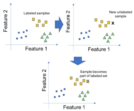
Self-training is the oldest form of semi-supervised learning [28]. It is an iterative process; during the first stage only la-beled data points are used by a supervised learning algorithm. Then, at each step, some of the unlabeled points are labeled according to the prediction resulting for the trained decision function and these points are used along with the original labeled data to retrain using the same supervised learning algorithm. This procedure is shown in Fig. 4.

Since the introduction of self-training, the idea of using la-beled and unlala-beled data has resulted in many semi-supervised

Fig. 4: Sample step of the self-training mechanism, where an unlabeled point is matched against labeled data to become part of the labeled data set.

learning algorithms. According to the classification proposed in [28], semi-supervised learning techniques can be organized in four classes: i) methods based on generative models4_{; ii)} methods based on the assumption that the decision boundary should lie in a low-density region; iii) graph-based methods; iv) two-step methods (first an unsupervised learning step to change the data representation or construct a new kernel; then a supervised learning step based on the new representation or kernel).

D. Reinforcement Learning

Reinforcement Learning (RL) is used, in general, to address applications such as robotics, finance (investment decisions), inventory management, where the goal is to learn a policy, i.e., a mapping between states of the environment into actions to be performed, while directly interacting with the environment. The RL paradigm allows agents to learn by exploring the available actions and refining their behavior using only an evaluative feedback, referred to as the reward. The agent’s goal is to maximize its long-term performance. Hence, the agent does not just take into account the immediate reward, but it evaluates the consequences of its actions on the future. Delayed reward and trial-and-error constitute the two most significant features of RL.

RL is usually performed in the context of Markov deci-sion processes (MDP). The agent’s perception at time k is represented as a state sk ∈ S, where S is the finite set of

environment states. The agent interacts with the environment by performing actions. At timek the agent selects an action

ak ∈ A, where A is the finite set of actions of the agent,

receive a reward as a result of the transition, according to the reward functionρ:S×A×S→R. The agents goal is to find the sequence of state-action pairs that maximizes the expected discounted reward, i.e., the optimal policy. In the context of MDP, it has been proved that an optimal deterministic and stationary policy exists. There exist a number of algorithms that learn the optimal policy both in case the state transition and reward functions are known (model-based learning) and in case they are not (model-free learning). The most used RL algorithm is Q-learning, a model-free algorithm that estimates the optimal action-value function (see chapter VI in [19]). An action-value function, named Qfunction, is the expected return of a state-action pair for a given policy. The optimal action-value function, Q∗, corresponds to the maximum expected return for a state-action pair. After learning function Q∗, the agent selects the action with the corresponding highest Q-value in correspondence to the current state.

A table-based solution such as the one described above is only suitable in case of problems with limited state-action space. In order to generalize the policy learned in correspondence to states not previously experienced by the agent, RL methods can be combined with existing function approximation methods, e.g., neural networks.

E. Overfitting, underfitting and model selection

In this section, we discuss a well-known problem of ML algorithms along with its solutions. Although we focus on supervised learning techniques, the discussion is also relevant for unsupervised learning methods.

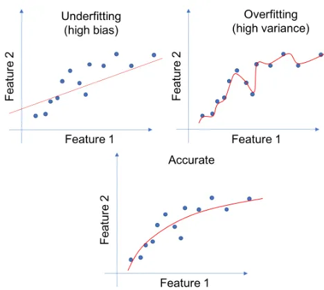
Overfitting and underfitting are two sides of the same coin: model selection. Overfitting happens when the model we use is too complex for the available dataset (e.g., a high polynomial order in the case of linear regression with polynomial basis functions or a too large number of hidden neurons for a neural network). In this case, the model will fit the training data too closely5_{, including noisy samples and outliers, but} will result in very poor generalization, i.e., it will provide inaccurate predictions for new data points. At the other end of the spectrum, underfitting is caused by the selection of models that are not complex enough to capture important features in the data (e.g., when we use a linear model to fit quadratic data). Fig. 5 shows the difference between underfitting and overfitting, compared to an accurate model.

Since the error measured on the training samples is a poor indicator for generalization, to evaluate the model performance the available dataset is split into two, the training set and the test set. The model is trained on the training set and then evaluated using the test set. Typically around 70% of the samples are assigned to the training set and the remaining30%

are assigned to the test set. Another option that is very useful in case of a limited dataset is to use cross-validation so that as much of the available data as possible is exploited for training. In this case, the dataset is divided into k subsets. The model 5_{As an extreme example, consider a simple regression problem for} pre-dicting a real-value target variable as a function of a real-value observation variable. Let us assume a linear regression model with polynomial basis function of the input variable. If we haveN samples and we selectN as the order of the polynomial, we can fit the model perfectly to the data points.

Fig. 5: Difference between underfitting and overfitting.

is trainedktimes using each of theksubset for validation and the remaining (k−1) subsets for training. The performance is averaged over the k runs. In case of overfitting, the error measured on the test set is high and the error on the training set is small. On the other hand, in the case of underfitting, both the error measured on the training set and the test set are usually high.

III. MOTIVATION FOR USING MACHINE LEARNING IN OPTICAL NETWORKS ANDSYSTEMS

In the last few years, the application of mathematical approaches derived from the ML discipline have attracted the attention of many researchers and practitioners in the optical communications and networking fields. In a general sense, the underlying motivations for this trend can be identified as follows:

• increased system complexity: the adoption of advanced transmission techniques, such as those enabled by coher-ent technology [11], and the introduction of extremely flexible networking principles, such as, e.g., the EON paradigm, have made the design and operation of optical networks extremely complex, due to the high number of tunable parameters to be considered (e.g., modulation formats, symbol rates, adaptive coding rates, adaptive channel bandwidth, etc.); in such a scenario, accurately modeling the system through closed-form formulas is often very hard, if not impossible, and in fact “margins” are typically adopted in the analytical models, leading to resource underutilization and to consequent increased system cost; on the contrary, ML methods can capture complex non-linear system behaviour with relatively sim-ple training of supervised and/or unsupervised algorithms which exploit knowledge of historical network data, and therefore to solve complex cross-layer problems, typical of the optical networking field;

• increased data availability: modern optical networks are equipped with a large number of monitors, able to provide several types of information on the entire system, e.g., traffic traces, signal quality indicators (such as BER), equipment failure alarms, users’ behaviour etc.; here, the enhancement brought by ML consists of simultaneously leveraging the plethora of collected data and discover hidden relations between various types of information. The application of ML to physical layer use cases is mainly motivated by the presence of non-linear effects in optical fibers, which make analytical models inaccurate or even too complex. This has implications, e.g., on the performance pre-dictions of optical communication systems, in terms of BER, quality factor (Q-factor) and also for signal demodulation [30], [31], [32].

Moving from the physical layer to the networking layer, the same motivation applies for the application of ML techniques. In particular, design and management of optical networks is continuously evolving, driven by the enormous increase of transported traffic and drastic changes in traffic requirements, e.g., in terms of capacity, latency, user experience and Quality of Service (QoS). Therefore, current optical networks are expected to be run at much higher utilization than in the past, while providing strict guarantees on the provided quality of service. While aggressive optimization and traffic-engineering methodologies are required to achieve these objectives, such complex methodologies may suffer scalability issues, and in-volve unacceptable computational complexity. In this context, ML is regarded as a promising methodological area to address this issue, as it enables automated network self-configuration

and fast decision-making by leveraging the plethora of data that can be retrieved via network monitors, and allowing net-work engineers to build data-driven models for more accurate and optimized network provisioning and management.

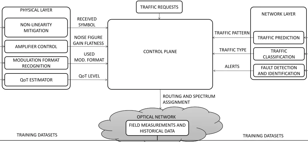
Several use cases can benefit from the application of ML and data analytics techniques. In this paper we divide these use cases ini)physical layerandii)network layeruse cases. The remainder of this section provides a high-level introduction to the main applications of ML in optical networks, as graphically shown in Fig. 6, and motivates why ML can be beneficial in each case. A detailed survey of existing studies is then provided in Sections IV and V, for physical layer and network layer use cases, respectively.

A. Physical layer domain

As mentioned in the previous section, several challenges need to be addressed at the physical layer of an optical net-work, typically to evaluate the performance of the transmission system and to check if any signal degradation influences existing lightpaths. Such monitoring can be used, e.g., to trigger proactive procedures, such as tuning of launch power, controlling gain in optical amplifiers, varying modulation format, etc., before irrecoverable signal degradation occurs. In the following, a description of the applications of ML at the physical layer is presented.

• QoT estimation.

Prior to the deployment of a new lightpath, a system engineer needs to estimate the Quality of Transmission (QoT) for the new lightpath, as well as for the already existing ones. The concept of Quality of Transmission generally refers to a number of physical layer param-eters, such as received Optical Signal-to-Noise Ratio (OSNR), BER, Q-factor, etc., which have an impact on the “readability” of the optical signal at the receiver. Such parameters give a quantitative measure to check if a pre-determined level of QoT would be guaranteed, and are affected by several tunable design parameters, such as, e.g., modulation format, baud rate, coding rate, physical path in the network, etc. Therefore, optimizing this choice is not trivial and often this large variety of possible parameters challenges the ability of a system engineer to address manually all the possible combinations of lightpath deployment.

NETWORK LAYER PHYSICAL LAYER

CONTROL PLANE NON-LINEARITY

MITIGATION

AMPLIFIER CONTROL

MODULATION FORMAT RECOGNITION

TRAFFIC PREDICTION

TRAFFIC CLASSIFICATION

QoT ESTIMATOR

OPTICAL NETWORK OPTICAL NETWORK FIELD MEASUREMENTS AND

HISTORICAL DATA

TRAINING DATASETS TRAINING DATASETS

TRAFFIC REQUESTS

ROUTING AND SPECTRUM ASSIGNMENT

TRAFFIC PATTERN

TRAFFIC TYPE

QoT LEVEL RECEIVED

SYMBOL

USED MOD. FORMAT NOISE FIGURE GAIN FLATNESS

FAULT DETECTION AND IDENTIFICATION ALERTS

Fig. 6: The general framework of a ML-assisted optical network.

system under consideration must be made in order to adopt approximate models. Conversely, ML constitutes a promising means to automatically predict whether un-established lightpaths will meet the required system QoT threshold.

Relevant ML techniques: ML-based classifiers can be trained using supervised learning6 _{to create direct} input-output relationship between QoT observed at the receiver and corresponding lightpath configuration in terms of, e.g., utilized modulation format, baud rate and/or physical route in the network.

• Optical amplifiers control.

In current optical networks, lightpath provisioning is becoming more dynamic, in response to the emergence of new services that require huge amount of bandwidth over limited periods of time. Unfortunately, dynamic set-up and tear-down of lightpaths over different wavelengths forces network operators to reconfigure network devices “on the fly” to maintain physical-layer stability. In re-sponse to rapid changes of lightpath deployment, Erbium Doped Fiber Amplifiers (EDFAs) suffer from wavelength-dependent power excursions. Namely, when a new light-path is established (i.e., added) or when an existing lightpath is torn down (i.e., dropped), the discrepancy of signal power levels between different channels (i.e., between lightpaths operating at different wavelengths) depends on the specific wavelength being added/dropped into/from the system. Thus, an automatic control of pre-amplification signal power levels is required, especially in case a cascade of multiple EDFAs is traversed, to avoid that excessive post-amplification power discrepancy

6_{Note that, specific solutions adopted in literature for QoT estimation, as} well as for other physical- and network-layer use cases, will be detailed in the literature surveys provided in Sections IV and V.

between different lightpaths may cause signal distortion.

Relevant ML techniques: Thanks to the availability of historical data retrieved by monitoring network status, ML regression algorithms can be trained to accurately predict post-amplifier power excursion in response to the add/drop of specific wavelengths to/from the system.

• Modulation format recognition (MFR).

Modern optical transmitters and receivers provide high flexibility in the utilized bandwidth, carrier frequency and modulation format, mainly to adapt the transmission to the required bit-rate and optical reach in a flexible/elastic networking environment. Given that at the transmission side an arbitrary coherent optical modulation format can be adopted, knowing this decision in advance also at the receiver side is not always possible, and this may affect proper signal demodulation and, consequently, signal processing and detection.

Relevant ML techniques: Use of supervised ML algo-rithms can help the modulation format recognition at the receiver, thanks to the opportunity to learn the mapping between the adopted modulation format and the features of the incoming optical signal.

• Nonlinearity mitigation.

Due to optical fiber nonlinearities, such as Kerr effect, self-phase modulation (SPM) and cross-phase modulation (XPM), the behaviour of several performance param-eters, including BER, Q-factor, Chromatic Dispersion (CD), Polarization Mode Dispersion (PMD), is highly unpredictable, and this may cause signal distortion at the receiver (e.g., I/Q imbalance and phase noise). Therefore, complex analytical models are often adopted to react to signal degradation and/or compensate undesired nonlinear effects.

models are usually adopted to solve such complex non-linear problems, supervised ML models can be designed to directly capture the effects of such nonlinearities, typi-cally exploiting knowledge of historical data and creating input-output relations between the monitored parameters and the desired outputs.

• Optical performance monitoring (OPM).

With increasing capacity requirements for optical com-munication systems, performance monitoring is vital to ensure robust and reliable networks. Optical performance monitoring aims at estimating the transmission parame-ters of the optical fiber system, such as BER, Q-factor, CD, PMD, during lightpath lifetime. Knowledge of such parameters can be then utilized to accomplish various tasks, e.g., activating polarization compensator modules, adjusting launch power, varying the adopted modula-tion format, re-route lightpaths, etc. Typically, optical performance parameters need to be collected at various monitoring points along the lightpath, thus large number of monitors are required, causing increased system cost. Therefore, efficient deployment of optical performance monitors in the proper network locations is needed to extract network information at reasonable cost.

Relevant ML techniques: To reduce the amount of mon-itors to deploy in the system, especially at intermediate points of the lightpaths, supervised learning algorithms can be used to learn the mapping between the optical fiber channel parameters and the properties of the detected signal at the receiver, which can be retrieved, e.g., by observing statistics of power eye diagrams, signal ampli-tude, OSNR, etc.

B. Network layer domain

At the network layer, several other use cases for ML arise. Provisioning of new lightpaths or restoration of existing ones upon network failure require complex and fast decisions that depend on several quickly-evolving data, since, e.g., oper-ators must take into consideration the impact onto existing connections provided by newly-inserted traffic. In general, an estimation of users’ and service requirements is desirable for an effective network operation, as it allows to avoid over-provisioning of network resources and to deploy resources with adequate margins at a reasonable cost. We identify the following main use cases.

• Traffic prediction.

Accurate traffic prediction in the time-space domain allows operators to effectively plan and operate their networks. In the design phase, traffic prediction allows to reduce over-provisioning as much as possible. During network operation, resource utilization can be optimized by performing traffic engineering based on real-time data, eventually re-routing existing traffic and reserving resources for future incoming traffic requests.

Relevant ML techniques: Through knowledge of his-torical data on users’ behaviour and traffic profiles in the time-space domain, a supervised learning algorithm can be trained to predict future traffic requirements and conse-quent resource needs. This allows network engineers to

activate, e.g., proactive traffic re-routing and periodical network re-optimization so as to accommodate all users traffic and simultaneously reduce network resources uti-lization.

Moreover, unsupervised learning algorithms can be also used to extract common traffic patterns in different por-tions of the network. Doing so, similar design and man-agement procedures (e.g., deployment and/or reservation of network capacity) can be activated also in different parts of the network, which instead show similarities in terms of traffic requirements, i.e., belonging to a same traffic profilecluster.

Note that, application of traffic prediction, and the rel-ative ML techniques, vary substantially according to the considered network segment (e.g., approaches for intra-datacenter networks may be different than those for access networks), as traffic characteristics strongly depend on the considered network segment.

• Virtual topology design (VTD) and reconfiguration.

The abstraction of communication network services by means of a virtual topology is widely adopted by network operators and service providers. This abstraction consists of representing the connectivity between two end-points (e.g., two data centers) via an adjacency in the virtual topology, (i.e., a virtual link), although the two end-points are not necessarily physically connected. After the set of all virtual links has been defined, i.e., after all the lightpath requests have been identified, VTD requires solving a Routing and Wavelength Assignment (RWA) problem for each lightpath on top of the underlying physical network. Note that, in general, many virtual topologies can co-exist in the same physical network, and they may represent, e.g., service required by different customers, or even different services, each with a specific set of requirements (e.g., in terms of QoS, bandwidth, and/or latency), provisioned to the same customer. VTD is not only necessary when a new service is pro-visioned and new resources are allocated in the network. In some cases, e.g., when network failures occur or when the utilization of network resources undergoes re-optimization procedures, existing(i.e., already-designed) virtual topologies shall be rearranged, and in these cases we refer to theVT reconfiguration.

To perform design and reconfiguration of virtual topolo-gies, network operators not only need to provision (or reallocate) network capacity for the required services, but may also need to provide additional resources according to the specific service characteristics, e.g., for guaran-teeing service protection and/or meeting QoS or latency requirements. This type of service provisioning is often referred to as network slicing, due to the fact that each provisioned service (i.e., each VT) represents a slice of the overall network.

virtual topologies (i.e.,network slices), thus enabling fast decision making and optimized resources provisioning, especially under dynamically-changing network condi-tions.

• Failure management.

When managing a network, the ability to perform failure detection and localization or even to determine the cause of network failure is crucial as it may enable operators to promptly perform traffic re-routing, in order to main-tain service status and meet Service Level Agreements (SLAs), and rapidly recover from the failure. Handling network failures can be accomplished at different levels. E.g., performing failure detection, i.e., identifying the set of lightpaths that were affected by a failure, is a relatively simple task, which allows network operators to only reconfigure the affected lightpaths by, e.g., re-routing the corresponding traffic. Moreover, the ability of performing also failure localization enables the activation of recovery procedures. This way, pre-failure network status can be restored, which is, in general, an optimized situation from the point of view of resources utilization. Furthermore, determining also the cause of network fail-ure, e.g., temporary traffic congestion, devices disruption, or even anomalous behaviour of failure monitors, is useful to adopt the proper restoring and traffic reconfiguration procedures, as sometimes remote reconfiguration of light-paths can be enough to handle the failure, while in some other cases in-field intervention is necessary. Moreover, prompt identification of the failure cause enables fast equipment repair and consequent reduction in Mean Time To Repair (MTTR).

Relevant ML techniques: ML can help handling the large amount of information derived from the continuous activity of a huge number of network monitors and alarms. E.g., ML classifiers algorithms can be trained to distinguish between regular and anomalous (i.e., de-graded) transmission. Note that, in such cases, semi-supervised approaches can be also used, whenever labeled data are scarce, but a large amount of unlabeled data is available. Further, ML classifiers can be trained to distinguish failure causes, exploiting the knowledge of previously observed failures.

• Traffic flow classification.

When different types of services coexist in the same network infrastructure, classifying the corresponding traf-fic flows before their provisioning may enable eftraf-ficient resource allocation, mitigating the risk of under- and over-provisioning. Moreover, accurate flow classification is also exploited for already provisioned services to apply flow-specific policies, e.g., to handle packets priority, to perform flow and congestion control, and to guarantee proper QoS to each flow according to the SLAs.

Relevant ML techniques: Based on the various traffic characteristics and exploiting the large amount of in-formation carried by data packets, supervised learning algorithms can be trained to extract hidden traffic charac-teristics and perform fast packets classification and flows differentiation.

• Path computation.

When performing network resources allocation for an incoming service request, a proper path should be se-lected in order to efficiently exploit the available network resources to accommodate the requested traffic with the desired QoS and without affecting the existing services, previously provisioned in the network. Traditionally, path computation is performed by using cost-based routing algorithms, such as Dijkstra, Bellman-Ford, Yen algo-rithms, which rely on the definition of a pre-defined cost metric (e.g., based on the distance between source and destination, the end-to-end delay, the energy con-sumption, or even a combination of several metrics) to discriminate between alternative paths.

Relevant ML techniques: In this context, use of su-pervised ML can be helpful as it allows to simultane-ously consider several parameters featuring the incoming service request together with current network state in-formation and map this inin-formation into an optimized routing solution, with no need for complex network-cost evaluations and thus enabling fast path selection and service provisioning.

C. A bird-eye view of the surveyed studies

The physical- and network-layer use cases described above have been tackled in existing studies by exploiting several ML tools (i.e., supervised and/or unsupervised learning, etc.) and leveraging different types of network monitored data (e.g., BER, OSNR, link load, network alarms, etc.).

In Tables I and II we summarize the various physical- and network-layer use cases and highlight the features of the ML approaches which have been used in literature to solve these problems. In the tables we also indicate specific reference papers addressing these issues, which will be described in the following sections in more detail. Note that another recently published survey [33] proposes a very similar categorization of existing applications of artificial intelligence in optical networks.

IV. DETAILED SURVEY OF MACHINE LEARNING IN PHYSICAL LAYER DOMAIN

A. Quality of Transmission estimation

QoT estimation consists of computing transmission quality metrics such as OSNR, BER, Q-factor, CD or PMD based on measurements directly collected from the field by means of optical performance monitors installed at the receiver side [105] and/or on lightpath characteristics. QoT estimation is typically applied in two scenarios:

• predicting the transmission quality of unestablished light-paths based on historical observations and measurements collected from already deployed ones;

• monitoring the transmission quality of already-deployed

lightpaths with the aim of identifying faults and malfunc-tions.

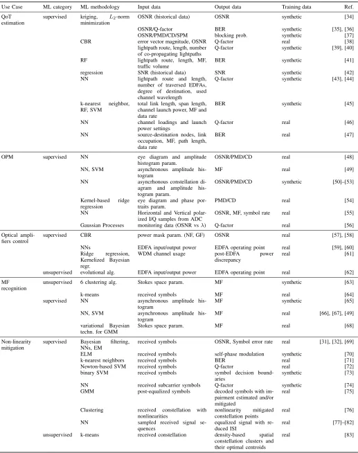
TABLE I: Different use cases at physical layer and their characteristics.

Use Case ML category ML methodology Input data Output data Training data Ref.

QoT estimation

supervised kriging, L2-norm

minimization

OSNR (historical data) OSNR synthetic [34]

OSNR/Q-factor BER synthetic [35], [36]

OSNR/PMD/CD/SPM blocking prob. synthetic [37]

CBR error vector magnitude, OSNR Q-factor real [38]

lightpath route, length, number of co-propagating lightpaths

Q-factor synthetic [39], [40]

RF lightpath route, length, MF,

traffic volume

BER synthetic [41]

regression SNR (historical data) SNR synthetic [42]

NN lightpath route and length,

number of traversed EDFAs, degree of destination, used channel wavelength

Q-factor synthetic [43], [44]

k-nearest neighbor, RF, SVM

total link length, span length, channel launch power, MF and data rate

BER synthetic [45]

NN channel loadings and launch

power settings

Q-factor real [46]

NN source-destination nodes, link occupation, MF, path length, data rate

BER real [47]

OPM supervised NN eye diagram and amplitude

histogram param.

OSNR/PMD/CD real [48]

NN, SVM asynchronous amplitude his-togram

MF real [49]

NN asyncrhonous constellation di-agram and amplitude his-togram param.

OSNR/PMD/CD synthetic [50]–[53]

Kernel-based ridge regression

eye diagram and phase por-traits param.

PMD/CD real [54]

NN Horizontal and Vertical polar-ized I/Q samples from ADC

OSNR, MF, symbol rate real [55]

Gaussian Processes monitoring data (OSNR vsλ) Q-factor real [56]

Optical ampli-fiers control

supervised CBR power mask param. (NF, GF) OSNR real [57], [58]

NNs EDFA input/output power EDFA operating point real [59], [60]

Ridge regression, Kernelized Bayesian regr.

WDM channel usage post-EDFA power

discrepancy

real [61]

unsupervised evolutional alg. EDFA input/output power EDFA operating point real [62]

MF recognition

unsupervised 6 clustering alg. Stokes space param. MF synthetic [63]

k-means received symbols MF real [64]

supervised NN asynchronous amplitude his-togram

MF synthetic [65]

NN, SVM asynchronous amplitude his-togram

MF real [66], [67], [49]

variational Bayesian techn. for GMM

Stokes space param. MF real [68]

Non-linearity mitigation

supervised Bayesian filtering, NNs, EM

received symbols OSNR, Symbol error rate real [31], [32], [69]

ELM received symbols self-phase modulation synthetic [70]

k-nearest neighbors received symbols BER real [71]

Newton-based SVM received symbols Q-factor real [72]

binary SVM received symbols symbol decision bound-aries

synthetic [73]

NN received subcarrier symbols Q-factor synthetic [74]

GMM post-equalized symbols decoded symbols with im-pairment estimated and/or mitigated

real [75]

Clustering received constellation with nonlinearities

nonlinearity mitigated constellation points

real [76]

NN sampled received signal

se-quences

equalized signal with re-duced ISI

real [77]–[82]

unsupervised k-means received constellation density-based spatial constellation clusters and their optimal centroids

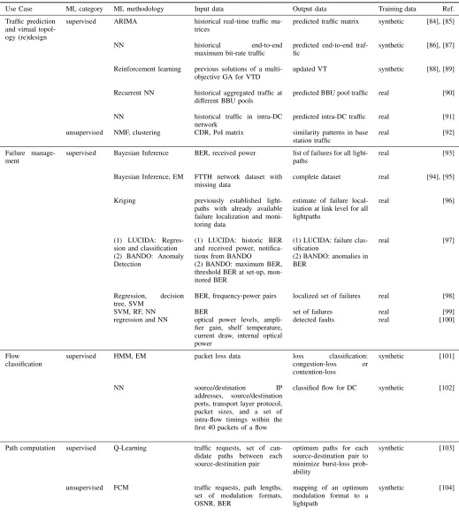
TABLE II: Different use cases at network layer and their characteristics.

Use Case ML category ML methodology Input data Output data Training data Ref.

Traffic prediction and virtual topol-ogy (re)design

supervised ARIMA historical real-time traffic ma-trices

predicted traffic matrix synthetic [84], [85]

NN historical end-to-end

maximum bit-rate traffic

predicted end-to-end traf-fic

synthetic [86], [87]

Reinforcement learning previous solutions of a multi-objective GA for VTD

updated VT synthetic [88], [89]

Recurrent NN historical aggregated traffic at different BBU pools

predicted BBU pool traffic real [90]

NN historical traffic in intra-DC network

predicted intra-DC traffic real [91]

unsupervised NMF, clustering CDR, PoI matrix similarity patterns in base station traffic

real [92]

Failure manage-ment

supervised Bayesian Inference BER, received power list of failures for all light-paths

real [93]

Bayesian Inference, EM FTTH network dataset with missing data

complete dataset real [94], [95]

Kriging previously established light-paths with already available failure localization and moni-toring data

estimate of failure local-ization at link level for all lightpaths

real [96]

(1) LUCIDA: Regres-sion and classification (2) BANDO: Anomaly Detection

(1) LUCIDA: historic BER and received power, notifica-tions from BANDO

(2) BANDO: maximum BER, threshold BER at set-up, mon-itored BER

(1) LUCIDA: failure clas-sification

(2) BANDO: anomalies in BER

real [97]

Regression, decision tree, SVM

BER, frequency-power pairs localized set of failures real [98]

SVM, RF, NN BER set of failures real [99]

regression and NN optical power levels, ampli-fier gain, shelf temperature, current draw, internal optical power

detected faults real [100]

Flow classification

supervised HMM, EM packet loss data loss classification:

congestion-loss or contention-loss

synthetic [101]

NN source/destination IP

addresses, source/destination ports, transport layer protocol, packet sizes, and a set of intra-flow timings within the first 40 packets of a flow

classified flow for DC synthetic [102]

Path computation supervised Q-Learning traffic requests, set of can-didate paths between each source-destination pair

optimum paths for each source-destination pair to minimize burst-loss prob-ability

synthetic [103]

unsupervised FCM traffic requests, path lengths, set of modulation formats, OSNR, BER

mapping of an optimum modulation format to a lightpath

synthetic [104]

will meet the required quality of service guarantees (mapped onto OSNR, BER or Q-factor threshold values): the problem is typically formulated as a binary classification problem, where the classifier outputs a yes/no answer based on the lightpath characteristics (e.g., its length, number of links, modulation format used for transmission, overall spectrum occupation of

the traversed links etc.).

deviation of the number of co-propagating lightpaths per link. Whenever a new traffic requests arrives, the most “similar” one (where similarity is computed by means of the Euclidean distance in the multidimensional space of normalized fea-tures) is retrieved from the database and a decision is made by comparing the associated Q-factor measurement with a predefined system threshold. As a correct dimensioning and maintenance of the database greatly affect the performance of the CBR technique, algorithms are proposed to keep it up to date and to remove old or useless entries. The trade-off between database size, computational time and effectiveness of the classification performance is extensively studied: in [40], the technique is shown to outperform state-of-the-art ML algorithms such as Naive Bayes, J48 tree and Random Forests (RFs). Experimental results achieved with data obtained from a real testbed are discussed in [38].

A database-oriented approach is proposed also in [42] to reduce uncertainties on network parameters and design margins, where field data are collected by a software defined network controller and stored in a central repository. Then, a QTool is used to produce an estimate of the field-measured Signal-to-Noise Ratio (SNR) based on educated guesses on the (unknown) network parameters and such guesses are iteratively updated by means of a gradient descent algorithm, until the difference between the estimated and the field-measured SNR falls below a predefined threshold. The new estimated parameters are stored in the database and yield to new design margins, which can be used for future demands. The trade-off between database size and ranges of the SNR estimation error are evaluated via numerical simulations.

Similarly, in the context of multicast transmission in optical network, a NN is trained in [43], [44], [46], [47] using as features the lightpath total length, the number of traversed EDFAs, the maximum link length, the degree of destination node and the channel wavelength used for transmission of candidate lightpaths, to predict whether the Q-factor will exceed a given system threshold. The NN is trained online with data mini-batches, according to the network evolution, to allow for sequential updates of the prediction model. A dropout technique is adopted during training to avoid overfitting. The classification output is exploited by a heuristic algorithm for dynamic routing and spectrum assignment, which decides whether the request must be served or blocked. The algorithm performance is assessed in terms of blocking probability.

A random forest binary classifier is adopted in [41] to predict the probability that the BER of unestablished lightpaths will exceed a system threshold. As depicted in Figure 7, the classifier takes as input a set of features including the total length and maximum link length of the candidate lightpath, the number of traversed links, the amount of traffic to be transmitted and the modulation format to be adopted for transmission. Several alternative combinations of routes and modulation formats are considered and the classifier identifies the ones that will most likely satisfy the BER requirements. In [45], a random forest classifier along with two other tools namely k-nearest neighbor and support vector machine are used. The authors in [45] use three of the above-mentioned classifiers to associate QoT labels with a large set of lightpaths

Fig. 7: The classification framework adopted in [41].

to develop a knowledge base and find out which is the best classifier. It turns out from the analysis in [45], that the support vector machine is better in performance than the other two but takes more computation time.

Two alternative approaches, namelynetwork kriging7 (first described in [107]) andnormL2minimization(typically used in network tomography [108]), are applied in [36], [37] in the context of QoT estimation: they rely on the installation of probe lightpaths that do not carry user data but are used to gather field measurements. The proposed inference methodologies exploit the spatial correlation between the QoT metrics of probes and data-carrying lightpaths sharing some physical links to provide an estimate of the Q-factor of already deployed or perspective lightpaths. These methods can be applied assuming either a centralized decisional tool or in a distributed fashion, where each node has only local knowledge of the network measurements. As installing probe lightpaths is costly and occupies spectral resources, the trade-off between number of probes and accuracy of the estimation is studied. Several heuristic algorithms for the placement of the probes are proposed in [34]. A further refinement of the methodologies which takes into account the presence of neighbor channels appears in [35].

Additionally, a data-driven approach using a machine learn-ing technique, Gaussian processes nonlinear regression (GPR), is proposed and experimentally demonstrated for performance prediction of WDM optical communication systems [49]. The core of the proposed approach (and indeed of any ML technique) is generalization: first the model is learned from the measured data acquired under one set of system configurations, and then the inferred model is applied to perform predictions for a new set of system configurations. The advantage of the approach is that complex system dynamics can be cap-tured from measured data more easily than from simulations. Accurate BER predictions as a function of input power, transmission length, symbol rate and inter-channel spacing are reported using numerical simulations and proof-of-principle experimental validation for a 24 × 28 GBd QPSK WDM optical transmission system.

Fig. 8: EDFA power mask [60].

Finally, a control and management architecture integrating an intelligent QoT estimator is proposed in [109] and its feasibility is demonstrated with implementation in a real testbed.

B. Optical amplifiers control

The operating point of EDFAs influences their Noise Figure (NF) and gain flatness (GF), which have a considerable impact on the overall ligtpath QoT. The adaptive adjustment of the operating point based on the signal input power can be accomplished by means of ML algorithms. Most of the existing studies [57]–[60], [62] rely on a preliminary amplifier characterization process aimed at experimentally evaluating the value of the metrics of interest (e.g., NF, GF and gain control accuracy) within its power mask (i.e., the amplifier operating region, depicted in Fig. 8).

The characterization results are then represented as a set of discrete values within the operation region. In EDFA im-plementations, state-of-the-art microcontrollers cannot easily obtain GF and NF values for points that were not measured during the characterization. Unfortunately, producing a large amount of fine grained measurements is time consuming. To address this issue, ML algorithms can be used to interpolate the mapping function over non-measured points.

For the interpolation, authors of [59], [60] adopt a NN im-plementing both feed-forward and backward error propagation. Experimental results with single and cascaded amplifiers re-port interpolation errors below 0.5 dB. Conversely, a cognitive methodology is proposed in [57], which is applied in dynamic network scenarios upon arrival of a new lightpath request: a knowledge database is maintained where measurements of the amplifier gains of already established lightpaths are stored, together with the lightpath characteristics (e.g., number of links, total length, etc.) and the OSNR value measured at the receiver. The database entries showing the highest similarities with the incoming lightpath request are retrieved, the vectors of gains associated to their respective amplifiers are considered and a new choice of gains is generated by perturbation of such

DP-BPSK DP-QPSK DP-8-QAM

Fig. 9: Stokes space representation of DP-BPSK, DP-QPSK and DP-8-QAM modulation formats [68].

values. Then, the OSNR value that would be obtained with the new vector of gains is estimated via simulation and stored in the database as a new entry. After this, the vector associated to the highest OSNR is used for tuning the amplifier gains when the new lightpath is deployed.

An implementation of real-time EDFA setpoint adjustment using the GMPLS control plane and interpolation rule based on a weighted Euclidean distance computation is described in [58] and extended in [62] to cascaded amplifiers.

Differently from the previous references, in [61] the issue of modelling the channel dependence of EDFA power excursion is approached by defining a regression problem, where the input feature set is an array of binary values indicating the occupation of each spectrum channel in a WDM grid and the predicted variable is the post-EDFA power discrepancy. Two learning approaches (i.e., the Ridge regression and Kernelized Bayesian regression models) are compared for a setup with 2 and 3 amplifier spans, in case of single-channel and superchan-nel add-drops. Based on the predicted values, suggestion on the spectrum allocation ensuring the least power discrepancy among channels can be provided.

C. Modulation format recognition

k = 2,4,8) and n-QAM (with n = 8,12,16) modulated signals.

Conversely, features extracted from asynchronous amplitude histograms sampled from the eye-diagram after equalization in digital coherent transceivers are used in [65]–[67] to train NNs. In [66], [67], a NN is used for hierarchical extraction of the amplitude histograms’ features, in order to obtain a compressed representation, aimed at reducing the number of neurons in the hidden layers with respect to the number of features. In [65], a NN is combined with a genetic algorithm to improve the efficiency of the weight selection procedure during the training phase. Both studies provide numerical results over experimentally generated data: the former obtains 0% error rate in discriminating among three modulation for-mats (PM-QPSK, 16-QAM and 64-QAM), the latter shows the tradeoff between error rate and number of histogram bins considering six different formats (OOK, ODB, NRZ-DPSK, RZ-DQPSK, PM-RZ-QPSK and PM-NRZ-16-QAM).

D. Nonlinearity mitigation

One of the performance metrics commonly used for optical communication systems is the data-rate×distance product. Due to the fiber loss, optical amplification needs to be em-ployed and, for increasing transmission distance, an increasing number of optical amplifiers must be employed accordingly. Optical amplifiers add noise and to retain the signal-to-noise ratio optical signal power is increased. However, increasing the optical signal power beyond a certain value will enhance optical fiber nonlinearities which leads to Nonlinear Inter-ference (NLI) noise. NLI will impact symbol detection and the focus of many papers, such as [31], [32], [69]–[73] has been on applying ML approaches to perform optimum symbol detection.

In general, the task of the receiver is to perform optimum symbol detection. In the case when the noise has circularly symmetric Gaussian distribution, the optimum symbol de-tection is performed by minimizing the Euclidean distance between the received symbolyk and all the possible symbols

of the constellation alphabet, s=sk|k= 1, ..., M. This type

of symbol detection will then have linear decision boundaries. For the case of memoryless nonlinearity, such as nonlinear phase noise, I/Q modulator and driving electronics nonlinear-ity, the noise associated with the symbolyk may no longer be

circularly symmetric. This means that the clusters in constel-lation diagram become distorted (elliptically shaped instead of circularly symmetric in some cases). In those particular cases, optimum symbol detection is no longer based on Euclidean distance matrix, and the knowledge and full parametrization of the likelihood function, p(yk|xk), is necessary. To determine

and parameterize the likelihood function and finally perform optimum symbol detection, ML techniques, such as SVM, kernel density estimator, k-nearest neighbors and Gaussian mixture models can be employed. A gain of approximately 3 dB in the input power to the fiber has been achieved, by employing Gaussian mixture model in combination with expectation maximization, for 14 Gbaud DP 16-QAM trans-mission over a 800 km dispersion compensated link [31].

Furthermore, in [71] a distance-weighted k-nearest neigh-bors classifier is adopted to compensate system impairments in zero-dispersion, dispersion managed and dispersion unman-aged links, with 16-QAM transmission, whereas in [74] NNs are proposed for nonlinear equalization in 16-QAM OFDM transmission (one neural network per subcarrier is adopted, with a number of neurons equal to the number of symbols). To reduce the computational complexity of the training phase, an Extreme Learning Machine (ELM) equalizer is proposed in [70]. ELM is a NN where the weights minimizing the input-output mapping error can be computed by means of a generalized matrix inversion, without requiring any weight optimization step.

SVMs are adopted in [72], [73]: in [73], a battery of log2(M) binary SVM classifiers is used to identify decision boundaries separating the points of a M-PSK constellation, whereas in [72] fast Newton-based SVMs are employed to mitigate inter-subcarrier intermixing in 16-QAM OFDM trans-mission.

All the above mentioned approaches lead to a 0.5-3 dB improvement in terms of BER/Q-factor.

In the context of nonlinearity mitigation or in general, impairment mitigation, there are a group of references that implement equalization of the optical signal using a variety of ML algorithms like Gaussian mixture models [75], clustering [76], and artificial neural networks [77]–[82]. In [75], the authors propose a GMM to replace the soft/hard decoder module in a PAM-4 decoding process whereas in [76], the authors propose a scheme for pre-distortion using the ML clustering algorithm to decode the constellation points from a received constellation affected with nonlinear impairments.

In references [77]–[82] that employ neural networks for equalization, usually a vector of sampled receive symbols act as the input to the neural networks with the output being equalized signal with reduced inter-symbol interference (ISI). In [77], [78], and [79] for example, a convolutional neural network (CNN) would be used to classify different classes of a PAM signal using the received signal as input. The number of outputs of the CNN will depend on whether it is a PAM-4, 8, or 16 signal. The CNN-based equalizers reported in [77]–[79] show very good BER performance with strong equalization capabilities.

While [77]–[79] report CNN-based equalizers, [81] shows another interesting application of neural network in impair-ment mitigation of an optical signal. In [81], a neural network approximates very efficiently the function of digital back-propagation (DBP), which is a well-known technique to solve the non-linear Schroedinger equation using split-step Fourier method (SSFM) [110]. In [80] too, a neural network is proposed to emulate the function of a receiver in a nonlinear frequency division multiplexing (NFDM) system. The pro-posed NN-based receiver in [80] outperforms a receiver based on nonlinear Fourier transform (NFT) and a minimum-distance receiver.