Unveiling the Linguistic Weaknesses
of Neural Machine Translation
my first encounter with
Back in 2014…
I had been working on word reordering models for five years
3
CHAPTER 5. MODIFIED DISTORTION MATRICES
!"#$%&''(#!)*#+,-.&)/01"2"3(#!**#45&67#,89:,;-<&0=>?77@"(#!7*#=+-,9&77"@*(#!7*#,8AB8C5D&0=>?77"2*(# !**#AD&67#.9,EF&77(#!7*#+;G,H&77(#!7*#,8,I"J&0=>?77*#,89,F=<&0=>?KK@"(#!**#8%&67#C-.<&77@"#LC&77*(#$%& ''#1;A&*M*2*3(#!)*#5CA8$D&)/*2*31"2*(#!7*#"$-&77(#!7*#,A5D&77(#!7*#B-&77(#!7*#,8C-.<&0=>?77@"(# !**#45&67#,804<&0=>?77*@"#,8N-F5<&0=>?KK@"#,8A=9I8&0=>?KK(#!**#45&67#,8BO$D&0=>?77#,8,B-,E585<&0=>?KK@"# A-$,D&77*#,8F-N$P5&0=>?77*(#Q&*R7'# $%#+,-.#45#,89:,;-<#=+-,9#,8AB8C5D#AD#.9,EF#+;G,S#,8,I"J#,89,F=<#8%#C-.<#LC#$%#1;A#5CA8$D#"$-#,A5D#B-# ,8C-.<#45#,804<#,8N-F5<#,8A=9I8#45#,8BO$D#,8,B-,E585<#A-$,D#,8F-N$P5#Q# 0TUVDB#T4#W-AVG#AVAFV-B#T4#9;V#/-XNWGVB#9TT.#<W-9#XD#9;V#GVATDB9-WYTD#WDG#ZW--XVG#[# ##$\######!"#$%%%%%%%&'%"()*"+#,%%%#=+-,9#,8AB8C5D#######AD#,8.9,EF#########Q###
#!"#$$$$%&&'$(!)%$$$$$*"$%+,$-!).+$$$$$#&/,"0$&1$-*2*%!"%0$$$1)&-$%+,$3)*4!#,0$$$$$$$#
#'']# ##)'^# *'3# 7'_# #*'`# #*Z9a# #'']# *'3# #)'^# 7'_# #*'`#
#)'^# *'3# 7'_#
#)'^# *'3# 7'_#
#)'^# *'3# 7'_# *'`#
#)'^# *'3# 7'_# *'`#
#'']# #'']# #'']# #'']# #*'`# #*'`# #*Z9a# #*Z9a# #*Z9a# #*Z9a# #*Z9a#
(a) Arabic VS(O) clause: five permutations
!"#$%&'! !((%&)! !"#$%&'! !((%&)!
!"#$%&'!
*&+! *&,! -&.!
*&+! *&,! -&.!
*&+! *&,! -&.! !((%&)!
!!-/01! !!-/01! !!-/01! *&+! !"#$%&'! *&,! -&.! !((%&)! !!-/01!
234!5#6"(470!-8974/#098:7!;</4!3"7!=>=?"046!=07!=>@47?A"?9>!9>!034!=>/=64>0B! C=4!5#6"(47048!D0""0!">E"F07/3"G!3"0!=384!H8I=JF#>A4>!K#I!%98L"FF!4=>A4F4=040!B!
M*&!C=4NOP2!5#6"(47048N**!D0""0N**!">E"F07/3"GN**Q!M%&!3"0N%ORS*Q!M*&!=384N--;DO2!H8I=JF#>A4>N**Q!M-&! K#INO--POP2!%98L"FFN**Q!M%&!4=>A4F4=040N%%--Q!BN-T*&!
C=4!5#6"(47048!D0""0!">E"F07/3"G!!!!!"#$!!!!!!=384!H8I=JF#>A4>!!!!K#I!%98L"FF!!!!!%&'(%)%&$%$!!!!!!B!!!!!!!!!!!
!!!!!!"#$!%&'()$*+!,-.*$/&+.-0*!12/$!!!!!!!!!!!!!#(*!!!!!!!!!!3+*!345$*67(6.4!!!!!!!!.4!+#$!(//3'$4+!!!!!!!3436(+$'!
(b) Germanbroken verb chunk: three permutations
Chunk types: CC conjunction, VC verb (auxiliary/past participle), PC preposition, NC noun, Pct punct.
Figure 5.1: Chunk permutations generated by fuzzy chunk-based reordering rules for translation into English.
vc and for each vc-punctuation sequence, at most 10 for each broken vc. Empirically, this yields on average 22 reorderings per sentence in the NIST-MT Arabic benchmark (dev06-nw) and 3 on the WMT German benchmark (test08).4 Arabic rules are indeed
more noisy, which is not surprising as all verb chunks can trigger some reordering. 5.3 Reordering selection
The number of chunk-based reorderings per sentence varies according to the rule set, the size of chunks, and the context. A high degree of fuzziness can complicate the decoding process, leaving too much work to the in-decoding reordering model. A solution to this problem is using an external model to score the rule-generated reorderings and discard the least likely. In such a way, a further part of reordering complexity is taken out of decoding.
At this end, instead of using a Support Vector Machine classifier as was done in Chapter 4, we apply reordered n-gram models that are lighter-weight and more suitable
4All benchmarks are described in detail in Section 5.5. 64
Computational Linguistics Volume xx, Number xx
Reordering models References Model Reordering step Features type classification
Phrase orientation models (POM):
Example:P(orient=discontinuous-left|next-phrase-pair=[jdd]-[renewed]) Tillmann 2004;
gener.
lexicalized (hierarchical) Koehn & al. 2005; source/target phrases phrase orientation model Nagata & al. 2006;
Galley & Manning 2008 monotonic, swap, phrase orientation
Zens & Ney 2006 discr. discontinuous
maxent classifier (left or right) source/target words sparse phrase Cherry 2013 discr. or word clusters orientation features
Jump models (JM):
Example:P(jump= 5|from=AlsAds,to=jdd) inbound/outbound/pairwise Al-Onaizan & Papineni
gener. jump length source words lexicalized distortion 2006
inbound/outbound
Green & al. 2010 discr. jump length based source words, POS, length-bin classifier (9 length bins) position; sent. length
Source decoding sequence models (SDSM):
Example:P(next-word=jdd|prev-translated-words=AlEahil Almlk mHmd AlsAds) reordered source n-gram Feng & al. 2010a gener. — source words
(9-gram context) source word-after-word
Bisazza & Federico 2013;
discr. —
source words, POS; Goto & al. 2013 source context’s words
and POS
Operation sequence models (OSM):
Example:P(next-operation=generate[jdd,renewed]|prev-operations=generate[AlsAds,VI] jumpBack[1]) translation/reordering Durrani & al. 2011;
gener.
insertGap, source/target words, operation n-gram Durrani & al. 2013; jumpBack, POS or word clusters;
Durrani & al. 2014 jumpForward prev.n–1 operations
Table 1: An overview of state-of-the-art reordering models for PSMT. Model type indicates whether a model is trained in a generative or discriminative way. All examples refer to the sentence pair shown in Figure 2.
Operation sequence models (OSM)(Durrani, Schmid, and Fraser 2011) are n-gram models that include lexical translation operations and reordering operations (insertGap,
jumpBack orjumpForward) in a single generative story, thereby combining elements from the previous three model families. An operation sequence example is provided in the lower part of Table 1. OSM are closely related to n-gram based SMT models (see next section) but have been successfully applied as feature functions to PSMT (Durrani et al. 2013). To overcome data sparseness, OSM can be successfully applied to POS-tags and unsupervised word clusters (Durrani et al. 2014).
SDSM and OSM have been proven optimal for language pairs where high distortion limits are required to capture long-range reordering phenomena (Durrani, Schmid, and Fraser 2011; Bisazza and Federico 2013b; Goto et al. 2013). Nevertheless POM remains the most widely used type of phrase-based reordering model and is considered a nec-essary component of PSMT baselines in any language pair. In particular, two variants 8
Bisazza and Federico A Survey of Word Reordering in Statistical Machine Translation
[jdd]3 [AlEAhl Almgrby]1 [Almlk mHmd AlsAds]2 [dEm -h]4 …!
[the Moroccan monarch]1 [King Mohamed VI]2 [renewed]3 [his support]4 …!
[jdd]3 [AlEAhl Almgrby]1 [Almlk mHmd AlsAds]2 [dEm -h]4 [l- m$rwE]5 [Alr}ys Alfrnsy]6!
[the Moroccan monarch]1 [King Mohamed VI]2 [renewed]3 [his support]4 [to the project of]5 [the French President]6!
hierarchical: swap!
[image:3.1024.524.944.225.599.2]standard: discontinuous!
Figure 3: Phrase orientation example for the phrase pair [jdd]-[renewed]: the standard model detects a discontinuous orientation with respect to the last translated phrase (2) whereas the hierarchical model detects a swap with respect to the block of phrases (1-2).
of POM deserve further attention because of their notable effect on translation quality: hierarchical POM and sparse phrase orientation features.
Hierarchical phrase orientation models, or simply hierarchical reordering models
(HRM) (Galley and Manning 2008) improve the way in which the orientation of a new phrase pair is determined: already translated adjacent blocks are merged together to form longer phrases around the current one. For instance in Figure 3, HRM merges phrases 1 and 2 into a large phrase pair [AlEahl ... AlsAds]-[The ... VI] and consequently
assigns a swap, instead of discontinuous orientation, to [jdd]-[renewed]. As a result, ori-entation assignments become more consistent across hypotheses with different phrase segmentations.
Rather than training a reordering model by relative frequency or maximum entropy and using its score as one dense feature function, Cherry (2013) introduces sparse
phrase orientation features that are directly added to the model score during decoding
(cf. equation (1)) and optimized jointly with all other SMT feature weights. Effective sparse reordering features can be obtained by simply coupling a phrase pair’s orienta-tion with the first or last word (or word class) of its source and target side (Cherry 2013), or even with the whole phrase pair identity (Auli, Galley, and Gao 2014).
2.2 N-gram based SMT
N-gram based SMT (Casacuberta and Vidal 2004; Mariño et al. 2006) is a string-based alternative to PSMT. In this framework, smoothed n-gram models are learnt over se-quences of minimal translation units (called tuples), which, like phrase pairs, are pairs of word sequences extracted from word-aligned parallel sentences. Tuples, however, are typically shorter than phrase pairs and are extracted from a unique,monotonic segmenta-tion of the sentence pair. Thus, the problem of spurious phrase segmentasegmenta-tion is avoided but non-local reordering becomes an issue. For instance, in Figure 2, a monotonic phrase segmentation could be achieved only by treating the large block [jdd ...
AlsAds]-[The ... renewed] as a single tuple. Reordering is then addressed by ‘tuple unfolding’
(Crego, Mariño, and de Gispert 2005): that is, during training the source words of each translation unit are rearranged in a target-like order so that more, shorter tuples can be extracted. At test time, input sentences have to bepre-orderedfor translation. To this end, Crego and Mariño (2006) propose to precompute a number of likely permutations of the input using POS-based rewrite rules learned during tuple unfolding. The reorderings thus obtained are used to extend the search graph of a monotonic decoder.8 Reordering
8 More pre-ordering techniques will be discussed in Section 2.4.
9
[image:3.1024.87.937.229.603.2]Back in 2014…
Montreal’s first NMT online demo:
4
EN-DE | EN-FR
Type text here:
The Budapest Prosecutor’s Office has initiated an investigation on the accident.
Translation:
New research direction
•
My interests suddenly switched to
discovering the strengths and
weaknesses
of neural seq(-to-seq) models
•
In 2016 published
first error analysis
of NMT vs SMT output post-editing
5
Auxiliary-main verb construction [aux:V]:
SRC in this experiment , individualswere shownhundreds of hours of YouTube videos
HPB in diesem Experiment , Individuengezeigt wurdenHunderte von Stunden YouTube-Videos
(a) PE in diesem Experimentwurden Individuen Hunderte von Stunden Youtube-Videosgezeigt NMT in diesem Experimentwurden Individuen hunderte Stunden YouTube Videosgezeigt PE in diesem Experimentwurden Individuen hunderte Stunden YouTube Videosgezeigt
Verb in subordinate (adjunct) clause [neb:V]:
SRC ... when coaches and managers and ownerslookat this information streaming ...
PBSY ... wenn Trainer und Manager und Eigent¨umerbetrachtendiese Information Streaming ...
(b) PE ... wenn Trainer und Manager und Eigent¨umer dieses Informations-Streaming betrachten... NMT ... wenn Trainer und Manager und Besitzer sich diese Informationenanschauen ...
PE ... wenn Trainer und Manager und Besitzer sich diese Informationenanschauen ...
Prepositional phrase [pp:PREP det:ART pn:N] acting as temporal adjunct:
SRC so like many of us , I ’ve lived in a few closetsin my life
SPB so wie viele von uns , ich habe in ein paar Schr¨ankein meinem Leben gelebt
(c) PE so habe ich wie viele von unsw¨ahrend meines Lebens in einigen Verstecken gelebt NMT wie viele von uns habe ich in ein paar Schr¨ankein meinem Leben gelebt
PE wie viele von uns habe ichin meinem Leben in ein paar Schr¨anken gelebt
Negation particle [adv:PTKNEG]:
SRC but I eventually came to the conclusion that that just didnot work for systematic reasons
HPB aber ich kam schlielich zu dem Schluss , dass nur aus systematischen Gr¨undennichtfunktionieren
(d) PE aber ich kam schlielich zu dem Schluss , dass es einfach aus systematischen Gr¨undennichtfunktioniert NMT aber letztendlich kam ich zu dem Schluss , dass das einfachnichtaus systematischen Gr¨unden funktionierte PE ich musste aber einsehen , dass das aus systematischen Gr¨undennicht funktioniert
Table 6: MT output and post-edit examples showing common types of reordering errors.
7 Conclusions
We analysed the output of four state-of-the-art MT systems that participated in the English-to-German task of the IWSLT 2015 evaluation campaign. Our selected runs were produced by three phrase-based MT systems and a neural MT system. The analysis leveraged high quality post-edits of the MT outputs, which allowed us to profile systems with respect to reliable measures of post-editing effort and transla-tion error types.
The outcomes of the analysis confirm that NMT has significantly pushed ahead the state of the art, especially in a language pair involving rich morphol-ogy prediction and significant word reordering. To summarize our findings: (i) NMT generates outputs that considerably lower the overall post-edit effort with respect to the best PBMT system (-26%); (ii)
NMT outperforms PBMT systems on all sentence lengths, although its performance degrades faster with the input length than its competitors; (iii) NMT seems to have an edge especially on lexically rich texts; (iv) NMT output contains less morphology
er-rors (-19%), less lexical erer-rors (-17%), and substan-tially less word order errors (-50%) than its closest competitor for each error type; (v) concerning word order, NMT shows an impressive improvement in the placement of verbs (-70% errors).
While NMT proved superior to PBMT with re-spect to all error types that were investigated, our analysis also pointed out some aspects of NMT that deserve further work, such as the handling of long sentences and the reordering of particular linguistic constituents requiring a deep semantic understand-ing of text. Machine translation is definitely not a solved problem, but the time is finally ripe to tackle its most intricate aspects.
Acknowledgments
FBK authors were supported by the CRACKER, QT21 and ModernMT projects, which received funding from the European Union’s Horizon 2020 programme under grants No. 645357, 645452 and 645487. AB was funded in part by the NWO under projects 639.022.213 and 612.001.218.
265
History repeats itself
6
SMT
ca.1990-2010
SMT+
ling. featuresca. 2005-2013 morph. segmentation
morph. inflection prediction CCG target features
feature-rich reordering models syntax-based preordering
tree-based SMT (various flavors)
SMT+
NN components2014 neural LMs
neural inflection prediction neural preordering
NMT
2015
MT solved
?
NMT+
ling. features
2017-2018 morph. segmentation
morph. inflection prediction
morph/POS/dep. source features CCG target features
tree-to-seq NMT
seq-to-(linearized)tree NMT translation+parsing as multitask
not really
Let’s take a step back
7
Do we know where we are going?
This time we’re dealing with a really black box
Research should aim at:
•
understanding the role played by linguistic structure in seq(-to-seq)
models
•
more systematic ways to know which linguistic phenomena are(n’t)
captured [
→
model interpretability ]
•
In pre-neural SMT we knew what could
not
work by model limitations (e.g. clearly flawed
independence assumptions)
•
Neural models have the potential to learn
Today’s talk
8
(1) What makes recurrent NNs work so well for language modeling?
(2) How important is recurrency for capturing hierarchical structure?
Part 1:
First Insights into the Workings of RNNs
10
Our first hypothesis: a great command of language structure (grammar)
How to find that out?
•
Augment an LSTM language model with a memory block (precursor to
self-attention)
•
Read out the weights of attention over the last
n
words
•
Test on language modeling: essential subtask of machine translation
and other seq-to-seq tasks
[Tran,Bisazza,Monz. NAACL’16]
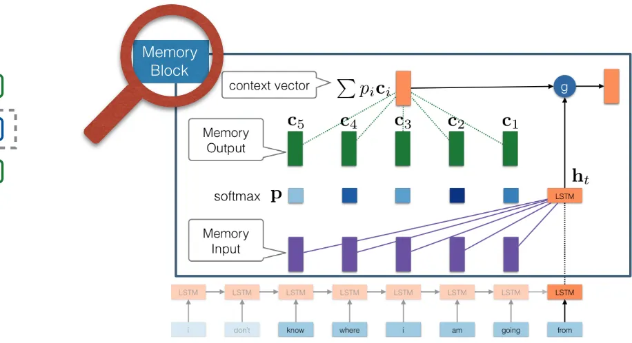
Recurrent Memory Network
know where i am going from
LSTM
Memory Block LSTM
ht
softmax
c1 c2
c3
c4
c5
p
g P
pici
End-to-end Memory Network (Sukhbaatar et. al) where zt is an update gate, rt is a reset gate.
The choice of the composition function g(·) is
crucial for the MB especially when one of its in-put comes from the LSTM. The simple addition function might overwrite the information within the LSTM’s hidden state and therefore prevent the MB from keeping track of information in the distant past. The gating function, on the other hand, can control the degree of information that flows from the LSTM to the MB’s output.
3.2 RMN Architectures
As explained above, our proposed MB receives the hidden state of the LSTM as one of its input. This leads to an intuitive combination of the two units by stacking the MB on top of the LSTM. We call this architecture Recurrent-Memory (RM). The RM ar-chitecture, however, does not allow interaction be-tween Memory Blocks at different time steps. To enable this interaction we can stack one more LSTM layer on top of the RM. We call this architecture Recurrent-Memory-Recurrent (RMR).
MB LSTM
LSTM LSTM
LSTM
MB LSTM
LSTM
MB MB
LSTM LSTM
[image:10.1024.423.881.450.699.2]LSTM LSTM MB
Figure 2: A graphical illustration of an unfolded RMR with memory size 4. Dashed line indicates concatenation. The MB takes the output of the bot-tom LSTM layer and the 4-word history as its input. The output of the MB is then passed to the second LSTM layer on top. There is no direct connection between MBs of different time steps. The last LSTM layer carries the MB’s outputs recurrently.
4 Language Model Experiments
Language models play a crucial role in many NLP applications such as machine translation and speech recognition. Language modeling also serves as a standard test bed for newly proposed models (Sukhbaatar et al., 2015; Kalchbrenner et al., 2015). We conjecture that, by explicitly accessing history words, RMNs will offer better predictive power than
the existing recurrent architectures. We therefore evaluate our RMN architectures against state-of-the-art LSTMs in terms of perplexity.
4.1 Data
We evaluate our models on three languages: En-glish, German, and Italian. We are especially inter-ested in German and Italian because of their larger vocabularies and complex agreement patterns. Ta-ble 1 summarizes the data used in our experiments.
Lang Train Dev Test |s| |V|
En 26M 223K 228K 26 77K
De 22M 202K 203K 22 111K
It 29M 207K 214K 29 104K
Table 1: Data statistics. |s| denotes the average
sen-tence length and |V| the vocabulary size.
The training data correspond to approximately 1M sentences in each language. For English, we use all the News Commentary data (8M tokens) and 18M tokens from News Crawl 2014 for train-ing. Development and test data are randomly drawn from the concatenation of the WMT 2009-2014 test sets (Bojar et al., 2015). For German, we use the first 6M tokens from the News Commentary data and 16M tokens from News Crawl 2014 for train-ing. For development and test data we use the re-maining part of the News Commentary data con-catenated with the WMT 2009-2014 test sets. Fi-nally, for Italian, we use a selection of 29M tokens from the PAIS `A corpus (Lyding et al., 2014), mainly including Wikipedia pages and, to a minor extent, Wikibooks and Wikinews documents. For develop-ment and test we randomly draw docudevelop-ments from the same corpus.
4.2 Setup
Our baselines are a 5-gram language model with Kneser-Ney smoothing, a Memory Network (MemN) (Sukhbaatar et al., 2015), a vanilla single-layer LSTM, and two stacked LSTMs with two and three layers respectively. N-gram models have been used intensively in many applications for their ex-cellent performance and fast training. Chen et al. (2015) show that n-gram model outperforms a pop-ular feed-forward language model (Bengio et al.,
11
Positional Analysis
de it enAttention visualization of 100 wor
d samples. Bottom positions in each
plot r
epr
esent most r
ecent histor
y. Darker color means higher weight.
A"en%on visualiza%on on 100 word samples (DE):
Average a"en%on per posi%on of RMN history:
Figure 3: Average attention per position of RMN
history. Top: RMR(–tM-g), bottom: RM(+tM-g).
Rightmost positions represent most recent history.
word) and decreases when moving further to the
left (less recent words). This is not surprising since
the success of
n
-gram language models has
demon-strated that the most recent words provide important
information for predicting the next word. Between
the two variants, the RM average attention mass is
less concentrated to the right. This can be explained
by the absence of an LSTM layer on top, meaning
that the MB in the RM architecture has to pay more
attention to the more distant words in the past. The
remaining analyses described below are performed
on the RM(+tM-g) architecture as this yields the best
perplexity results overall.
Beyond average attention weights, we are
inter-ested in those cases where attention focuses on
dis-tant positions. To this end, we randomly sample 100
words from test data and visualize attention
distri-butions over the last 15 words. Figure 4 shows the
attention distributions for random samples of
Ger-man and Italian. Again, in Ger-many cases attention
weights concentrate around the last word (bottom
row). However, we observe that many long distance
words also receive noticeable attention mass.
Inter-estingly, for many predicted words, attention is
dis-tributed evenly over memory positions, possibly
in-de
it
en
Figure 4: Attention visualization of 100 word
sam-ples. Bottom positions in each plot represent most
recent history. Darker color means higher weight.
dicating cases where the LSTM state already
con-tains enough information to predict the next word.
To explain the long-distance dependencies, we
first hypothesize that our RMN mostly memorizes
frequent co-occurrences. We run the RM(+tM-g)
model on the German development and test
sen-tences, and select those pairs of (
most-attended-word, word-to-predict
) where the MB’s attention
concentrates on a word more than six positions to
the left. Then, for each set of pairs with equal
dis-tance, we compute the mean frequency of
corre-sponding co-occurrences seen in the training data
(Table 3). The lack of correlation between frequency
and memory location suggests that RMN does more
than simply memorizing frequent co-occurrences.
d 7 8 9 10 11 12 13 14 15
µ 54 63 42 67 87 47 67 44 24
Table 3: Mean frequency (
µ
) of (
most-attended-word, word-to-predict
) pairs grouped by relative
dis-tance (
d
).
Previous work (Hermans and Schrauwen, 2013;
Karpathy et al., 2015) studied this property of
LSTMs by analyzing simple cases of closing
brack-ets. By contrast RMN allows us to discover more
interesting dependencies in the data. We manually
inspect those high-frequency pairs to see whether
they display certain linguistic phenomena. We
ob-serve that RMN captures, for example,
separable
verbs
and
fixed expressions
in German. Separable
verbs are frequent in German: they typically consist
of preposition+verb constructions, such
ab+h¨angen
(‘to depend’) or
aus+schließen
(‘to exclude’), and
can be spelled together (
abh¨angen
) or apart as in
‘
h¨angen von der Situation ab
’ (‘depend on the
sit-uation’), depending on the grammatical
construc-tion. Figure 5a shows a long-dependency
exam-ple for the separable verb
abh¨angen (to depend)
.
When predicting the verb’s particle
ab
, the model
correctly attends to the verb’s core
h¨angt
occurring
seven words to the left. Figure 5b and 5c show fixed
expression examples from German and Italian,
re-spectively:
schl¨usselrolle ... spielen (play a key role)
and
insignito ... titolo (awarded title)
. Here too, the
model correctly attends to the key word despite its
long distance from the word to predict.
326
Figure 3: Average attention per position of RMN history. Top: RMR(–tM-g), bottom: RM(+tM-g). Rightmost positions represent most recent history.
word) and decreases when moving further to the left (less recent words). This is not surprising since the success of n-gram language models has
demon-strated that the most recent words provide important information for predicting the next word. Between the two variants, the RM average attention mass is less concentrated to the right. This can be explained by the absence of an LSTM layer on top, meaning that the MB in the RM architecture has to pay more attention to the more distant words in the past. The remaining analyses described below are performed on the RM(+tM-g) architecture as this yields the best perplexity results overall.
Beyond average attention weights, we are inter-ested in those cases where attention focuses on dis-tant positions. To this end, we randomly sample 100 words from test data and visualize attention distri-butions over the last 15 words. Figure 4 shows the attention distributions for random samples of Ger-man and Italian. Again, in Ger-many cases attention weights concentrate around the last word (bottom row). However, we observe that many long distance words also receive noticeable attention mass. Inter-estingly, for many predicted words, attention is dis-tributed evenly over memory positions, possibly
in-de
it
en
Figure 4: Attention visualization of 100 word sam-ples. Bottom positions in each plot represent most recent history. Darker color means higher weight.
dicating cases where the LSTM state already con-tains enough information to predict the next word.
To explain the long-distance dependencies, we first hypothesize that our RMN mostly memorizes frequent co-occurrences. We run the RM(+tM-g) model on the German development and test sen-tences, and select those pairs of ( most-attended-word, word-to-predict) where the MB’s attention concentrates on a word more than six positions to the left. Then, for each set of pairs with equal dis-tance, we compute the mean frequency of corre-sponding co-occurrences seen in the training data (Table 3). The lack of correlation between frequency and memory location suggests that RMN does more than simply memorizing frequent co-occurrences.
d 7 8 9 10 11 12 13 14 15
µ 54 63 42 67 87 47 67 44 24
Table 3: Mean frequency (µ) of (
most-attended-word, word-to-predict) pairs grouped by relative dis-tance (d).
Previous work (Hermans and Schrauwen, 2013; Karpathy et al., 2015) studied this property of LSTMs by analyzing simple cases of closing brack-ets. By contrast RMN allows us to discover more interesting dependencies in the data. We manually inspect those high-frequency pairs to see whether they display certain linguistic phenomena. We ob-serve that RMN captures, for example, separable verbs and fixed expressions in German. Separable verbs are frequent in German: they typically consist of preposition+verb constructions, such ab+h¨angen
(‘to depend’) or aus+schließen (‘to exclude’), and can be spelled together (abh¨angen) or apart as in ‘h¨angen von der Situation ab’ (‘depend on the sit-uation’), depending on the grammatical construc-tion. Figure 5a shows a long-dependency exam-ple for the separable verb abh¨angen (to depend). When predicting the verb’s particle ab, the model correctly attends to the verb’s core h¨angt occurring seven words to the left. Figure 5b and 5c show fixed expression examples from German and Italian, re-spectively: schl¨usselrolle ... spielen (play a key role)
and insignito ... titolo (awarded title). Here too, the model correctly attends to the key word despite its long distance from the word to predict.
326
First Insights into the Workings of RNNs
ab(-1.8)
und (-2.1) , (-2.5) . (-2.7) von (-2.8)
(a) wie wirksam die daraus resultierende strategie sein wird , hängt daher von der genauigkeit dieser annahmen
Gloss: how effective the from-that resulting strategy be will, depends therefore on the accuracy of-these measures
Translation: how effective the resulting strategy will be, therefore, depends on the accuracy of these measures
spielen (-1.9)
gewinnen (-3.0)
finden (-3.4)
haben (-3.4)
schaffen (-3.4) … die lage versetzen werden , eine schlüsselrolle bei der eindämmung der regionalen ambitionen chinas zu
Gloss: … the position place will, a key-role in the curbing of-the regional ambitions China’s to Translation: …which will put him in a position to play a key role in curbing the regional ambitions of China
(b)
sacro (-1.5)
titolo(-2.9)
re(-3.0)
<unk>(-3.1) leone(-3.6)
... che fu insignito nel 1692 dall' Imperatore Leopoldo I del
Gloss: … who was awarded in 1692 by-the Emperor Leopold I of-the
Translation: … who was awarded the title by Emperor Leopold I in 1692
(c)
Figure 5: Examples of distant memory positions attended by RMN. The resulting top five word predictions are shown with the respective log-probabilities. The correct choice (in bold) was ranked first in sentences (a,b) and second in (c).
Other interesting examples found by the RMN in the test data include:
German: findet statt (takes place), kehrte zur¨uck
(came back), fragen antworten (questions
answers), k¨ampfen gegen (fight against), bleibt erhalten (remains intact), verantwortung
¨ubernimmt (takes responsibility);
Italian: sinistra destra (left right), latitudine lon-gitudine (latitude longitude), collegata tramite
(connected through), spos`o figli (got-married
children), insignito titolo (awarded title).
5.2 Syntactic analysis
It has been conjectured that RNNs, and LSTMs in particular, model text so well because they capture syntactic structure implicitly. Unfortunately this has been hard to prove, but with our RMN model we can get closer to answering this important question.
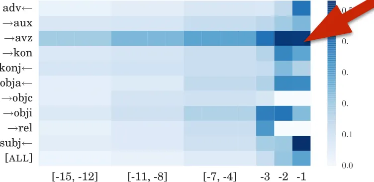
We produce dependency parses for our test sets using (Sennrich et al., 2013) for German and (At-tardi et al., 2009) for Italian. Next we look at how much attention mass is concentrated by the RM(+tM-g) model on different dependency types. Figure 6 shows, for each language, a selection of ten dependency types that are often long-distance.2 Dependency direction is marked by an arrow: e.g.
!mod means that the word to predict is a modifier
of the attended word, while mod means that the
2The full plots are available at https://github.com/
ketranm/RMN. The German and Italian tag sets are explained in (Simi et al., 2014) and (Foth, 2006) respectively.
attended word is a modifier of the word to predict.3 White cells denote combinations of position and de-pendency type that were not present in the test data. While in most of the cases closest positions are attended the most, we can see that some dependency types also receive noticeably more attention than the average (ALL) on the long-distance positions.
In German, this is mostly visible for the head of separable verb particles (!avz), which nicely sup-ports our observations in the lexical analysis (Sec-tion 5.1). Other attended dependencies include: aux-iliary verbs (!aux) when predicting the second el-ement of a complex tense (hat . . . gesagt / has said); subordinating conjunctions (konj ) when predict-ing the clause-final inflected verb (dass sie sagen sollten / that they should say); control verbs (!obji) when predicting the infinitive verb (versucht ihr zu helfen / tries to help her). Out of the Italian dependency types selected for their frequent long-distance occurrences (bottom of Figure 6), the most attended are argument heads (!arg), complement heads (!comp), object heads (!obj) and subjects (subj ). This suggests that RMN is mainly captur-ing predicate argument structure in Italian. Notice that syntactic annotation is never used to train the model, but only to analyze its predictions.
We can also use RMN to discover which complex dependency paths are important for word prediction. To mention just a few examples, high attention on
3Some dependency directions, like obj in Italian, are
al-most never observed due to order constraints of the language.
327
Long-dependency examples:
First Insights into the Workings of RNNs
12 [Tran,Bisazza,Monz. NAACL’16]
Lexical co-occurrences
Lexical analysis
61"
61" Neural"language"modeling"meets"linguis1c"intui1on"
Lexical Analysis
German English Trans
findet statt takes place
kehrte zuruck came back
fragen antworten questions answers
kämpfen gegen fight against
bleibt erhalten remains intact
verantwortung übernimmt takes responsibility
Lexical Analysis
Italian English Trans
sinistra destra left right
latitudine longitudine latitude longitude collegata tramite connected through sposò figli got-married children insignito titolo awarded title
Frequent"pairs"of"(most_aRended_word,(predicted_word)"with" distance">6"words:"
RMN"can"capture"relevant"coQoccurrences"regardless"of"distance"
Frequent pairs of mostAttendedWord-predictedWord with distance >6 words:
Syntactic dependencies
•only to a limited extent
•
mostly separable verbs
(in German)
?
Later work [Linzen & al. 2016] confirmed and explained our findings:
[image:12.1024.479.855.394.577.2]LSTM captures long syntactic dependencies
iff
explicit supervision is used
[-15, -12] [-11, -8] [-7, -4] -3 -2 -1
[ALL] subj!
rel
!obji !objc
obja konj!
kon
!avz !aux
adv
0.0
0.1
0.
0.
0.
0.5
Figure 6: Average attention weights per position, broken down by dependency relation type+direction between the attended word and the word to predict. Top: German. Bottom: Italian. More distant posi-tions are binned.
the German path [subj ,!kon,!cj] indicates that the model captures morphological agreement be-tween coordinate clauses in non-trivial constructions of the kind: spielen die Kinder im Garten und singen / the children play in the garden and sing. In Italian, high attention on the path [!obj,!comp,!prep]
denotes cases where the semantic relatedness be-tween a verb and its object does not stop at the ob-ject’s head, but percolates down to a prepositional phrase attached to it (pass`o buona parte della sua vita / spent a large part of his life). Interestingly, both local n-gram context and immediate depen-dency context would have missed these relations.
While much remains to be explored, our analysis shows that RMN discovers patterns far more com-plex than pairs of opening and closing brackets, and suggests that the network’s hidden state captures to a large extent the underlying structure of text.
6 Sentence Completion Challenge
The Microsoft Research Sentence Completion Chal-lenge (Zweig and Burges, 2012) has recently
be-come a test bed for advancing statistical language modeling. We choose this task to demonstrate the effectiveness of our RMN in capturing sentence co-herence. The test set consists of 1,040 sentences se-lected from five Sherlock Holmes novels by Conan Doyle. For each sentence, a content word is removed and the task is to identify the correct missing word among five given candidates. The task is carefully designed to be non-solvable for local language mod-els such as n-gram models. The best reported
re-sult is 58.9% accuracy (Mikolov et al., 2013)4 which is far below human accuracy of 91% (Zweig and Burges, 2012).
As baseline we use a stacked three-layer LSTM. Our models are two variants of RM(+tM-g), each consisting of three LSTM layers followed by a MB. The first variant (unidirectional-RM) uses n
words preceding the word to predict, the second (bidirectional-RM) uses the n words preceding and
the n words following the word to predict, as MB
input. We include bidirectional-RM in the experi-ments to show the flexibility of utilizing future con-text in RMN.
We train all models on the standard training data of the challenge, which consists of 522 novels from Project Gutenberg, preprocessed similarly to (Mnih and Kavukcuoglu, 2013). After sentence splitting, tokenization and lowercasing, we randomly select 19,000 sentences for validation. Training and val-idation sets include 47M and 190K tokens respec-tively. The vocabulary size is about 64,000.
We initialize and train all the networks as de-scribed in Section 4.2. Moreover, for regularization, we place dropout (Srivastava et al., 2014) after each LSTM layer as suggested in (Pham et al., 2014). The dropout rate is set to 0.3 in all the experiments.
Table 4 summarizes the results. It is worth to mention that our LSTM baseline outperforms a de-pendency RNN making explicit use of syntactic in-formation (Mirowski and Vlachos, 2015) and per-forms on par with the best published result (Mikolov et al., 2013). Our unidirectional-RM sets a new state of the art for the Sentence Completion Challenge with 69.2% accuracy. Under the same setting of d
we observe that using bidirectional context does not
4The authors use a weighted combination of skip-ngram and
RNN without giving any technical details.
Part 2:
How important is recurrency
Recently a family of non-recurrent models show competitive performance
on seq-to-seq modeling, esp. machine translation:
•
CNNs
(Convolutional Neural Networks) [Gehring & al. 2017]
•
FANs
(Fully Attentional Networks) [Vaswani & al. 2017]
The Importance of Being Recurrent
14
[Tran,Bisazza,Monz. arXiv 2018]
But does this kind of models capture hierarchical structure?
Capturing hierarchical structure is necessary to truly understand, process
and translate language
2 100 101 102 103 104 105 106 107 108 109 110 111 112 113 114 115 116 117 118 119 120 121 122 123 124 125 126 127 128 129 130 131 132 133 134 135 136 137 138 139 140 141 142 143 144 145 146 147 148 149 150 151 152 153 154 155 156 157 158 159 160 161 162 163 164 165 166 167 168 169 170 171 172 173 174 175 176 177 178 179 180 181 182 183 184 185 186 187 188 189 190 191 192 193 194 195 196 197 198 199 NAACL-HLT 2018 Submission 755. Confidential Review Copy. DO NOT DISTRIBUTE.
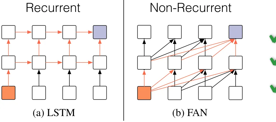
(a) LSTM (b) FAN
Figure 1: Diagram of the main difference between an LSTM and a FAN. The purple box indicates the
summarized vector at current time step t which is
used to make prediction. Orange arrows indicate the information flow from a previous input to that vector.
For the details of self-attention mechanics in
FANs, we refer to the work of Vaswani et al. (2017).
We now proceed to measure both models’ ability to learn hierarchical structure with a set of controlled experiments.
3 Tasks
We choose two tasks to study in this work: (1) subject-verb agreement, and (2) logical inference.
The first task was proposed by Linzen et al. (2016)
to test the ability of recurrent neural networks to capture syntactic dependencies in natural language.
The second task was introduced by Bowman et al.
(2015b) to compare tree-based recursive neural net-works against sequence-based recurrent netnet-works with respect to their ability to exploit hierarchical structures to make accurate inferences. The choice of tasks here is important to ensure that both mod-els have to exploit hierarchical structural features (Jia and Liang, 2017).
4 Subject-Verb Agreement
Linzen et al. (2016) propose the task of predict-ing number agreement between subject and verb in naturally occurring English sentences as a proxy for the ability of LSTMs to capture hierarchical structure in natural language. We use the dataset
provided by Linzen et al. (2016) and follow their
experimental protocol of training each model us-ing either (a) a general language model, i.e., next word prediction objective, and (b) an explicit super-vision objective, i.e., predicting the number of the
verb given its sentence history. Table 1 illustrates
the training and testing conditions of the task.
[image:14.1024.176.661.330.545.2]Data: Following the original setting, we take 10% of the data for training, 1% for validation, and the rest for testing. The vocabulary consists of the 10k
Table 1: Examples of training and test conditions for the two subject-verb agreement subtasks. The
full input sentence is “The keys to the cabinet are
on the table” where verb and subject are bold and distractor words are underlined.
Input Train Test
(a) the keys to the cabinet are p(are) > p(is)?
(b) the keys to the cabinet plural plural/singular?
most frequent words, while the remaining words are replaced by their part-of-speech.
Hyperparameters: In this experiment, both the LSTM and the FAN have 4 layers, the dropout rate is 0.2, and word-embeddings and hidden sizes are set to 128. The weights of the word embed-dings and output layer are shared as suggested by
Inan et al. (2017); Press and Wolf (2017). The FAN has 2 attention heads. LSTMs are trained with the Adam optimizer with a learning rate of 0.001. The FAN is trained with Adam for the language model objective and the YellowFin
op-timizer (Zhang et al., 2017)1 for the number
pre-diction objective. The initial learning rate is set to 0.001.
We first assess whether the LSTM and FAN models trained with respect to the language model objective assign higher probabilities to the
cor-rectly inflected verbs. As shown by Figures 2a
and 2b, both models achieve high accuracies for
this task, but LSTMs consistently outperform FANs. Moreover, LSTMs are clearly more ro-bust than FANs with respect to task difficulty, mea-sured both in terms of word distance and number
of agreement attractors2 between subject and verb.
Interestingly, Christiansen and Chater (2016);
Cor-nish et al. (2017) have argued that human memory limitations give rise to important characteristics of natural language, including its hierarchical struc-ture. Similarly, our experiments suggest that, by compressing the history into a single vector before making predictions, LSTMs are forced to better learn the input structure. On the other hand, de-spite having direct access to all words in their his-tory, FANs are less capable of detecting the verb’s subject. We note that the validation perplexities of the LSTM and FAN are 75.17 and 71.39,
respec-1We found that YellowFin gives better results than Adam
for FANs.
2Agreement attractors are intervening nouns with the
op-posite number from the subject.
Recurrent Non-Recurrent
Lower complexity
Much more parallelizable
We choose two tasks where capturing hierarchical structure is strictly
required:
•
subject-verb agreement
[Linzen & al. 2016]:
The Importance of Being Recurrent
15
(2) The keys to the cabinet are on the table.
Given a syntactic parse of the sentence and a verb, it is straightforward to identify the head of the subject that corresponds to that verb, and use that information to determine the number of the verb (Figure 1).
The keys to the cabinet are on the table
det
nsubj
prep pobjdet prep pobjdet
root
Figure 1: The form of the verb is determined by the head of the subject, which is directly connected to it via an nsubj edge. Other nouns that intervene between the head of the subject and the verb (here cabinet is such a noun) are irrelevant for determining the form of the verb and need to be ignored.
By contrast, models that are insensitive to structure may run into substantial difficulties capturing this de-pendency. One potential issue is that there is no limit to the complexity of the subject NP, and any number of sentence-level modifiers and parentheticals—and therefore an arbitrary number of words—can appear between the subject and the verb:
(3) The building on the far right that’s quite old
and run down is the Kilgore Bank Building.
This property of the dependency entails that it can-not be captured by an n-gram model with a fixed n.
RNNs are in principle able to capture dependencies of an unbounded length; however, it is an empirical question whether or not they will learn to do so in practice when trained on a natural corpus.
A more fundamental challenge that the depen-dency poses for structure-insensitive models is the possibility of agreement attraction errors (Bock and Miller, 1991). The correct form in (3) could be se-lected using simple heuristics such as “agree with the most recent noun”, which are readily available to sequence models. In general, however, such heuris-tics are unreliable, since other nouns can intervene between the subject and the verb in the linear se-quence of the sentence. Those intervening nouns can have the same number as the subject, as in (4), or the opposite number as in (5)-(7):
(4) Alluvial soils carried in the floodwaters add
nutrients to the floodplains.
(5) The only championship banners that are cur-rently displayed within the building are for national or NCAA Championships.
(6) The length of the forewings is 12-13.
(7) Yet the ratio of men who survive to the women and children who survive is not clear in this story.
Intervening nouns with the opposite number from the subject are called agreement attractors. The potential presence of agreement attractor entails that the model must identify the head of the syntactic subject that corresponds to a given verb in order to choose the correct inflected form of that verb.
Given the difficulty in identifying the subject from the linear sequence of the sentence, dependencies such as subject-verb agreement serve as an argument for structured syntactic representations in humans (Everaert et al., 2015); they may challenge models such as RNNs that do not have pre-wired syntac-tic representations. We note that subject-verb num-ber agreement is only one of a numnum-ber of structure-sensitive dependencies; other examples include nega-tive polarity items (e.g., any) and reflexive pronouns (herself). Nonetheless, a model’s success in learning subject-verb agreement would be highly suggestive of its ability to master hierarchical structure.
3 The Number Prediction Task
To what extent can a sequence model learn to be sensi-tive to the hierarchical structure of natural language? To study this question, we propose the number pre-diction task. In this task, the model sees the sentence up to but not including a present-tense verb, e.g.:
(8) The keys to the cabinet
It then needs to guess the number of the following verb (a binary choice, either PLURAL or SINGULAR).
We examine variations on this task in Section 5.
In order to perform well on this task, the model needs to encode the concepts of syntactic number and syntactic subjecthood: it needs to learn that some words are singular and others are plural, and to be able to identify the correct subject. As we have
illus-4 300 301 302 303 304 305 306 307 308 309 310 311 312 313 314 315 316 317 318 319 320 321 322 323 324 325 326 327 328 329 330 331 332 333 334 335 336 337 338 339 340 341 342 343 344 345 346 347 348 349 350 351 352 353 354 355 356 357 358 359 360 361 362 363 364 365 366 367 368 369 370 371 372 373 374 375 376 377 378 379 380 381 382 383 384 385 386 387 388 389 390 391 392 393 394 395 396 397 398 399 NAACL-HLT 2018 Submission 755. Confidential Review Copy. DO NOT DISTRIBUTE.
( d ( or f ) ) A ( f ( and a ) ) ( d ( and ( c ( or d ) ) ) ) # ( not f )
( not ( d ( or ( f ( or c ) ) ) ) ) @ ( not ( c ( and ( not d ) ) ) )
Why artificial data?
Despite the simplicity of the
language, this task is not trivial. To correctly
clas-sify logical relations, the model must learn nested
structures as well as the scope of logical
oper-ations. We verify the difficulty of the task by
training three bag-of-words models followed by
sum/average/max-pooling. The best of the three
models achieve less than 59% accuracy on the
log-ical inference versus 77% on the Stanford
Natu-ral Language Inference (SNLI) corpus (
Bowman
et al.
,
2015a
). This shows that the SNLI task can be
largely solved by exploiting shallow features
with-out understanding the underlying linguistic
struc-tures.
5.1 Models
We follow the general architecture proposed in
(
Bowman et al.
,
2015b
): Premise and hypothesis
sentences are encoded by fixed-size vectors. These
two vectors are then concatenated and fed to a
3-layer feed-forward neural network with ReLU
non-linearities to perform 7-way classification.
The LSTM architecture used in this experiment
is similar to that of
Bowman et al.
(
2015b
). We
simply take the last hidden state of the top LSTM
layer as a fixed-size vector representation of the
sentence. Here we use a 2-layer LSTM with skip
connections. The FAN maps a sentence
x
of length
n
to
H
= [
h
1, . . . ,
h
n]
2
R
d⇥n. To obtain a
fixed-size representation
z
, we use a self-attention layer
with two trainable queries
q
1,
q
22
R
1⇥d:
z
i=
softmax
✓
q
iH
p
d
◆
H
>i
2
{
1
,
2
}
z
= [
z
1,
z
2]
5.2 Results
Following the experimental protocol of
Bowman
et al.
(
2015b
), the data is divided into 13 bins based
on the number of logical operations. Both FANs
and LSTMs are trained on samples with at most
n
logical operations and tested on all bins. Figure
4
shows the result of the experiments with
n
6
and
n
12
. We see that FANs and LSTMs perform
similarly when trained on the whole dataset
(Fig-ure
4b
). However when trained on a subset of the
(a) n 6
(b) n 12
Figure 4: Results of logical inference
data (Figure
4a
), LSTMs obtain better accuracies
on similar examples (
n
6
) and LSTMs
general-ize better on longer examples (
6
< n
12
).
6 Discussion and Conclusion
We have compared a recurrent architecture (LSTM)
to a non-recurrent one (FAN) with respect to the
ability of capturing hierarchical structure. Our
ex-periments show that LSTMs slightly but
consis-tently outperform FANs. We found that LSTMs
are notably more robust with respect to the
pres-ence of misleading features in the agreement task,
whether trained with explicit supervision or with
a general language model objective. Finally, we
found that LSTMs generalize better to longer
se-quences for the logical inference task. These
find-ings suggest that recurrency is a key model
prop-erty which should not be sacrificed for efficiency
when hierarchical structure matters for the task.
This does not imply that LSTMs should
al-ways be preferred over non-recurrent architectures.
In fact, both FAN- and CNN-based networks
have proved to perform comparably or better than
LSTM-based ones on a very complex task like
ma-chine translation (
Gehring et al.
,
2017
;
Vaswani
et al.
,
2017
). Nevertheless, we believe that the
abil-ity of capturing hierarchical information in
sequen-tial data remains a fundamental need for building
intelligent systems that can understand and process
language. Thus we hope that our insights will be
useful towards building the next generation of
neu-ral networks.
• Predict 1 of 7 logical relations • Artificial data
•
logical inference
[Bowman & al. 2015]:
[Tran,Bisazza,Monz. arXiv 2018]
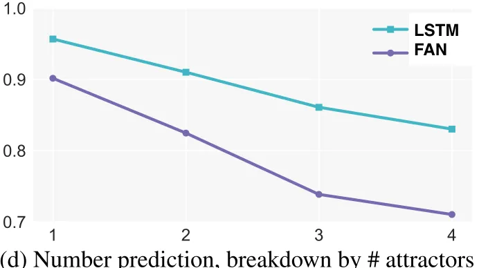
Results(1) Subject-Verb Agreement
16
•
Both models achieve high performance
•
LSTM slightly but consistently better and more robust to task difficulty
•
(FAN has lower perplexity though)
[Tran,Bisazza,Monz. arXiv 2018]
3 200 201 202 203 204 205 206 207 208 209 210 211 212 213 214 215 216 217 218 219 220 221 222 223 224 225 226 227 228 229 230 231 232 233 234 235 236 237 238 239 240 241 242 243 244 245 246 247 248 249 250 251 252 253 254 255 256 257 258 259 260 261 262 263 264 265 266 267 268 269 270 271 272 273 274 275 276 277 278 279 280 281 282 283 284 285 286 287 288 289 290 291 292 293 294 295 296 297 298 299 NAACL-HLT 2018 Submission 755. Confidential Review Copy. DO NOT DISTRIBUTE.
(a) Language model, breakdown by distance (b) Language model, breakdown by # attractors
[image:16.1024.116.893.100.473.2](c) Number prediction, breakdown by distance (d) Number prediction, breakdown by # attractors
Figure 2: Results of subject-verb agreement with different training objectives.
tively. The lack of correlation between perplex-ity and agreement accuracy indicates that FANs might capture other aspects of language better than LSTMs. We leave this question to future work.
Second, we evaluate FAN and LSTM models explicitly trained to predict the verb number (Fig-ures 2c and 2d) Again, we observe that LSTMs consistently outperform FANs. This is a partic-ularly interesting result since the self-attention mechanism in FANs connects two words in any po-sition with a O(1) number of executed operations, whereas RNNs require more recurrent operations. Despite this apparent advantage of FANs, the per-formance gap between FANs and LSTMs increases with the distance and number of attractors.3
To gain further insights into our results, we ex-amine the attention weights computed by FANs during verb-number prediction (supervised objec-tive). Specifically, for each attention head at each layer of the FAN, we compute the percentage of times the subject is the most attended word among all words in the history. Figure 3 shows the results for all cases where the model made the correct pre-diction. While it is hard to interpret the exact role of attention for different heads and at different lay-ers, we find that some of the attention heads at the higher layers (l3-h1, l2-h0) frequently point to the subject with an accuracy that decreases linearly
3We note that our LSTM results are better than those in
(Linzen et al., 2016). Also surprising is that the language model objective yields higher accuracies than the number pre-diction objective. We believe this may be due to better model optimization and to the embedding-output layer weight shar-ing, but we leave a thorough investigation to future work.
Figure 3: Proportion of times the subject is the most attended word by different heads at different layers (l3 is the highest layer). Only cases where the model made a correct prediction are shown.
with the distance between subject and verb.
5 Logical inference
In this task, we choose the artificial language in-troduced by Bowman et al. (2015b). This lan-guage has six word types {a, b, c, d, e, f} and three logical operations {or, and, not}. There are seven mutually exclusive logical relations that de-scribe the relationship between two sentences: en-tailment (@, A), equivalence (⌘), exhaustive and non-exhaustive contradiction (^, |), and two types
of semantic independence (#, `). We generate 60,000 samples4 with the number of logical op-erations ranging from 1 to 12. The train/dev/test dataset ratios are set to 0.8/0.1/0.1. In the follow-ing, we show some samples of the training data.
[image:16.1024.528.874.257.451.2]Results(2) Logical Inference
17
•
Similar performance when trained on whole data
•
LSTM much better than FAN when only trained on short sequences
(generalization power)
[Tran,Bisazza,Monz. arXiv 2018]
4 300 301 302 303 304 305 306 307 308 309 310 311 312 313 314 315 316 317 318 319 320 321 322 323 324 325 326 327 328 329 330 331 332 333 334 335 336 337 338 339 340 341 342 343 344 345 346 347 348 349 350 351 352 353 354 355 356 357 358 359 360 361 362 363 364 365 366 367 368 369 370 371 372 373 374 375 376 377 378 379 380 381 382 383 384 385 386 387 388 389 390 391 392 393 394 395 396 397 398 399 NAACL-HLT 2018 Submission 755. Confidential Review Copy. DO NOT DISTRIBUTE.
( d ( or f ) ) A ( f ( and a ) ) ( d ( and ( c ( or d ) ) ) ) # ( not f )
( not ( d ( or ( f ( or c ) ) ) ) ) @ ( not ( c ( and ( not d ) ) ) )
Why artificial data? Despite the simplicity of the language, this task is not trivial. To correctly clas-sify logical relations, the model must learn nested structures as well as the scope of logical oper-ations. We verify the difficulty of the task by training three bag-of-words models followed by sum/average/max-pooling. The best of the three models achieve less than 59% accuracy on the log-ical inference versus 77% on the Stanford Natu-ral Language Inference (SNLI) corpus (Bowman et al., 2015a). This shows that the SNLI task can be largely solved by exploiting shallow features with-out understanding the underlying linguistic struc-tures.
5.1 Models
We follow the general architecture proposed in (Bowman et al., 2015b): Premise and hypothesis sentences are encoded by fixed-size vectors. These two vectors are then concatenated and fed to a 3-layer feed-forward neural network with ReLU non-linearities to perform 7-way classification.
The LSTM architecture used in this experiment is similar to that of Bowman et al. (2015b). We simply take the last hidden state of the top LSTM layer as a fixed-size vector representation of the sentence. Here we use a 2-layer LSTM with skip connections. The FAN maps a sentence x of length n to H = [h1, . . . ,hn] 2 Rd⇥n. To obtain a
fixed-size representation z, we use a self-attention layer
with two trainable queries q1,q2 2 R1⇥d:
zi = softmax
✓
qiH p
d
◆
H> i 2 {1,2}
z = [z1, z2]
5.2 Results
Following the experimental protocol of Bowman et al. (2015b), the data is divided into 13 bins based on the number of logical operations. Both FANs and LSTMs are trained on samples with at most n logical operations and tested on all bins. Figure 4 shows the result of the experiments with n 6 and
n 12. We see that FANs and LSTMs perform
similarly when trained on the whole dataset (Fig-ure 4b). However when trained on a subset of the
(a) n 6
[image:17.1024.518.878.253.451.2](b) n 12
Figure 4: Results of logical inference
data (Figure 4a), LSTMs obtain better accuracies on similar examples (n 6) and LSTMs
general-ize better on longer examples (6 < n 12).
6 Discussion and Conclusion
We have compared a recurrent architecture (LSTM) to a non-recurrent one (FAN) with respect to the ability of capturing hierarchical structure. Our ex-periments show that LSTMs slightly but consis-tently outperform FANs. We found that LSTMs are notably more robust with respect to the pres-ence of misleading features in the agreement task, whether trained with explicit supervision or with a general language model objective. Finally, we found that LSTMs generalize better to longer se-quences for the logical inference task. These find-ings suggest that recurrency is a key model prop-erty which should not be sacrificed for efficiency when hierarchical structure matters for the task.
This does not imply that LSTMs should al-ways be preferred over non-recurrent architectures. In fact, both FAN- and CNN-based networks have proved to perform comparably or better than LSTM-based ones on a very complex task like ma-chine translation (Gehring et al., 2017; Vaswani et al., 2017). Nevertheless, we believe that the abil-ity of capturing hierarchical information in sequen-tial data remains a fundamental need for building intelligent systems that can understand and process language. Thus we hope that our insights will be useful towards building the next generation of neu-ral networks. 4 300 301 302 303 304 305 306 307 308 309 310 311 312 313 314 315 316 317 318 319 320 321 322 323 324 325 326 327 328 329 330 331 332 333 334 335 336 337 338 339 340 341 342 343 344 345 346 347 348 349 350 351 352 353 354 355 356 357 358 359 360 361 362 363 364 365 366 367 368 369 370 371 372 373 374 375 376 377 378 379 380 381 382 383 384 385 386 387 388 389 390 391 392 393 394 395 396 397 398 399 NAACL-HLT 2018 Submission 755. Confidential Review Copy. DO NOT DISTRIBUTE.
( d ( or f ) ) A ( f ( and a ) ) ( d ( and ( c ( or d ) ) ) ) # ( not f )
( not ( d ( or ( f ( or c ) ) ) ) ) @ ( not ( c ( and ( not d ) ) ) )
Why artificial data? Despite the simplicity of the language, this task is not trivial. To correctly clas-sify logical relations, the model must learn nested structures as well as the scope of logical oper-ations. We verify the difficulty of the task by training three bag-of-words models followed by sum/average/max-pooling. The best of the three models achieve less than 59% accuracy on the log-ical inference versus 77% on the Stanford Natu-ral Language Inference (SNLI) corpus (Bowman et al., 2015a). This shows that the SNLI task can be largely solved by exploiting shallow features with-out understanding the underlying linguistic struc-tures.
5.1 Models
We follow the general architecture proposed in (Bowman et al., 2015b): Premise and hypothesis sentences are encoded by fixed-size vectors. These two vectors are then concatenated and fed to a 3-layer feed-forward neural network with ReLU non-linearities to perform 7-way classification.
The LSTM architecture used in this experiment is similar to that of Bowman et al. (2015b). We simply take the last hidden state of the top LSTM layer as a fixed-size vector representation of the sentence. Here we use a 2-layer LSTM with skip connections. The FAN maps a sentence x of length n to H = [h1, . . . ,hn] 2 Rd⇥n. To obtain a
fixed-size representation z, we use a self-attention layer
with two trainable queries q1,q2 2 R1⇥d:
zi = softmax
✓
qiH p
d
◆
H> i 2 {1, 2}
z = [z1,z2]
5.2 Results
Following the experimental protocol of Bowman et al. (2015b), the data is divided into 13 bins based on the number of logical operations. Both FANs and LSTMs are trained on samples with at most n logical operations and tested on all bins. Figure 4 shows the result of the experiments with n 6 and
n 12. We see that FANs and LSTMs perform
similarly when trained on the whole dataset (Fig-ure 4b). However when trained on a subset of the
(a) n 6
(b) n 12
Figure 4: Results of logical inference
data (Figure 4a), LSTMs obtain better accuracies on similar examples (n 6) and LSTMs
general-ize better on longer examples (6 < n 12).
6 Discussion and Conclusion
We have compared a recurrent architecture (LSTM) to a non-recurrent one (FAN) with respect to the ability of capturing hierarchical structure. Our ex-periments show that LSTMs slightly but consis-tently outperform FANs. We found that LSTMs are notably more robust with respect to the pres-ence of misleading features in the agreement task, whether trained with explicit supervision or with
a general language model objective. Finally, we found that LSTMs generalize better to longer se-quences for the logical inference task. These find-ings suggest that recurrency is a key model prop-erty which should not be sacrificed for efficiency when hierarchical structure matters for the task.
This does not imply that LSTMs should al-ways be preferred over non-recurrent architectures. In fact, both FAN- and CNN-based networks have proved to perform comparably or better than LSTM-based ones on a very complex task like ma-chine translation (Gehring et al., 2017; Vaswani et al., 2017). Nevertheless, we believe that the abil-ity of capturing hierarchical information in sequen-tial data remains a fundamental need for building intelligent systems that can understand and process language. Thus we hope that our insights will be useful towards building the next generation of neu-ral networks.
LSTM FAN
Part 3:
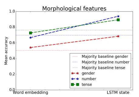
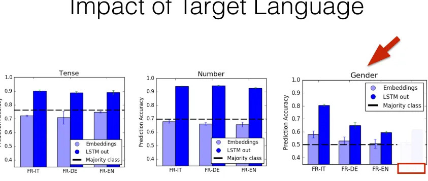
Morphological features in NMT embeddings
Potential: understand if injecting linguistic knowledge into machine translation
(e.g. via supervised annotation) is a promising direction
•
Specifically, we look at morphology on the source side
•
Build on and extend first analysis by [Belinkov & al. 2017]
•
Method: Train linguistic classifiers on word representations produced by
NMT encoders
19
[Bisazza,Tump. In Preparation]
Classifier
(lstm-state)
singular?
plural?
Classifier
(embedding)
singular?
plural?
https://aws.amazon.com/blogs/machine-learning
![Figure 3: Phrase orientation example for the phrase pair5 . 3Re o r de r i ngs e l e ct i o n [jdd]-[renewed]: the standardmodel detects a discontinuous orientation with respect to the last translated phrase (2)translation/reorderingwhereas the hierarchical model detects a swap with respect to the block of phrases (1-2).operation n-gram](https://thumb-us.123doks.com/thumbv2/123dok_us/1452683.683012/3.1024.524.944.225.599/orientation-standardmodel-discontinuous-orientation-translated-translation-reorderingwhereas-hierarchical.webp)