HEvAS: Headline Evaluation and Analysis System

Proceedings of the Multiling 2019 Workshop, co-located with the RANLP 2019 conference, pages 73–80 Varna, Bulgaria, September 6, 2019.

73

HEvAS: Headline Evaluation and Analysis System

Marina Litvak, Natalia Vanetik, Itzhak Eretz Kdosha

Software Engineering Department, Shamoon College of Engineering,

Beer Sheva, Israel

{marinal,natalyav,itzhaer}@ac.sce.ac.il

Abstract

Automatic headline generation is a sub-task of one-line summarization with many reported applications. Evaluation of sys-tems generating headlines is a very chal-lenging and undeveloped area. We intro-duce the Headline Evaluation and Anal-ysis System (HEvAS) that performs au-tomatic evaluation of systems in terms of a quality of the generated headlines. HEvAS provides two types of metrics– one which measures the informativeness of a headline, and another that measures its readability. The results of evaluation can be compared to the results of base-line methods which are implemented in HEvAS. The system also performs the sta-tistical analysis of the evaluation results and provides different visualization charts. This paper describes all evaluation met-rics, baselines, analysis, and architecture, utilized by our system.

1 Introduction

A headline of a document can be defined as a short sentence that gives a reader a general idea about the main contents of the story it entitles. There have been many reported practical applications for

headline generation (Colmenares et al., 2015) or

related tasks. Automatic evaluation of automat-ically generated headlines is a highly important task, where a candidate headline is assessed with respect to (1) readability (i.e. whether the head-line is easy to understand), and (2) relevance (i.e. whether the headline reflects the main topic of an article). Building unbiased metrics that manage to make objective evaluations of these properties has been proved to be a difficult task. Some of the related work resort to human-assisted

evalua-tion (Zajic et al.,2002), which is undoubtedly

ex-pensive and time-consuming. Therefore, most of works rely on the existing tools for automatic

eval-uation such as ROUGE (Shen et al.,2016;Hayashi

and Yanagimoto,2018). The main assumption be-ing that because the metrics work well for stan-dard summaries, the same applicable to short sum-maries and headlines, as a private case. However,

authors of (Colmenares et al., 2015) provide

sta-tistical evidence that this statement does not neces-sarily hold. We suspect that the main reason is that a summary needs to convey the content of a doc-ument while a headline should introduce, but not describe, the main subject of a document. More-over, even very short summaries usually include at least two full sentences while headlines do not. Despite that discovery, not many attempts to de-velop special metrics for the headline evaluation were made. Two new metrics—an adaptation of a ROUGE metric, and a metric for comparing head-lines on a conceptual level using Latent Semantic

Indexing (LSI) —were introduced in (Colmenares

et al.,2015).

2 Related Work

This section surveys the metrics used recently in literature for a headline evaluation task and ap-proaches we use for the introduced metrics as part of HEvAS. For the rest of this paper the terms “ref-erence headline” and “candidate headline” will be used to address the human-generated and the au-tomatically generated headlines, respectively.

2.1 ROUGE metrics

ROUGE metrics (Lin, 2004) are widely used for

evaluation of summaries, aiming to identify con-tent overlap—in terms of word n-grams—between gold-standard (reference) summaries and the eval-uated (system) summary.

This recall-oriented metric measures the number

ofN-grams in the reference headline that are also

present in a candidate headline. It is defined as:

|n-grams(R)∩n-grams(C)|

|n-grams(R)| ,whereRrefers to the

ref-erence headline,C to the candidate headline, and

the function n-gramsreturns the set of

contigu-ousN-grams of words in a text. In our system we

use the ROUGE-N metric withN = 1andN = 2.

ROUGE-SU

One of the problems of using the ROUGE-N

met-ric (withN > 1) is that requesting headlines to

share contiguousN-grams might be a very strong

condition. This is even more problematic when taking into account that headlines are comprised,

on average, of8-10tokens. This metric combines

ROUGE-1 with a relaxed version of ROUGE-2 that takes into account non-contiguous (skip)

bi-grams. For example,“President Trump said”will

produce three skip bigrams: “President Trump,”

“President said,”and“Trump said.” Let’s denote a function that returns all unigrams of the

head-line H as 1-grams(H), and a function that

re-turns its skip-bigrams ass2-grams(H). Then

for-mally,ROU GE-SU(R, C)is defined as follows:

|su(R)∩su(C)|

|su(R)| , wheresu(H) = 1-grams(H) ∪

s2-grams(H). By allowing gaps between

bi-grams, this metric detects similarities among phrases that differ by adjectives, or small changes.

ROUGE-WSU

The main problem of ROUGE-SU is that it gives the same importance to all skip-bigrams extracted from a phrase. For instance, suppose that the

fol-lowing phrases were compared:H1 :“x B C x x”,

H2 : “B y y y C”, H3 : “z z B z C”. The

only skip-bigram they all have in common is

“B-C,”, and ROUGE-SU gives us the same

simi-larity score between the three of them.

Au-thors of (Colmenares et al., 2015) proposed to

weight the skip-bigrams with respect to their av-erage skip-distance. Formally, it must be

calcu-lated as:

P

(a,b)∈su(R)∩su(C)

2

distR(a,b)+_distC(a,b)

P

(a,b)∈su(R) 1

distR(a,b)

where

functiondistH(a, b)returns the skip distance

be-tween words“a”and“b” in headlineH. For

un-igrams, the function returns1. This measure

pro-duces different scores forH2andH3in our

exam-ple. Namely, ROUGE-WSU(H1, H3)>

ROUGE-WSU(H1, H2).

2.2 Averaged Kullback–Leibler divergence

The Kullback–Leibler divergence is a measure of how two probability distributions are different. It is widely used for measuring the similarity be-tween texts, as the distance bebe-tween the proba-bility distributions of their words. However, the KL-divergence is not symmetric and cannot be used as a distance metric. Therefore, the averaged KL-divergence is used instead, which is defined

as follows (Huang, 2008): DAvgKL(t~a||t~b) =

Pm

t=1(π1 × D(wt,a||wt) + π2 × D(wt,b||wt)),

wheret~ais a vector representation of a text

(doc-ument or headline in our case)a,wt,ais a weight1

of term t in a text a, π1 = _wt,awt,a_+wt,b, π2 =

wt,b

wt,a+wt,b, andwt=π1×wt,a+π2×wt,b.

2.3 Latent Semantic Indexing

The ROUGE and KL-Divergence metrics relate two headlines only on the basis of word co-occurrences, i.e., they compare headlines at a very

low syntactic level (token matching). We also

need other metrics that are able to detect abstract concepts in the text and useful for both compar-ing headlines at a semantic level and measurcompar-ing of a headline’s coverage of a document topics. For

this end, authors of (Colmenares et al.,2015)

de-cided to use Latent Semantic Indexing (LSI) to ex-tract latent concepts from a corpus and represent documents as vectors in this abstract space. The similarity was then computed by means of angu-lar distances. The exact steps that were performed in (Colmenares et al., 2015), are as follows: (1)

a document-TF-IDF matrixM is built; (2)

Singu-lar Value Decomposition (SVD) is performed on

M resulting in matricesU SVT; (3) the

eigenval-ues in matrixS are analyzed and filtered; (4) the

transformation matrixV S−1 is calculated, which

enables the translation of TF-IDF document vec-tors to vecvec-tors in latent space; (5) after computing latent space vectors for both the headline and the entire document, their cosine similarity is calcu-lated.

2.4 Topic Modeling

Topic model is a type of statistical model for dis-covering the abstract “topics” that occur in a col-lection of documents. Latent Dirichlet allocation

(LDA) (Blei et al.,2003;Blei, 2012) allows

doc-uments to have a mixture of topics. LDA uses a

1_The

generative probabilistic approach for discovering the abstract topics, (i.e., clusters of semantically coherent documents). In particular, we define a

word as the basic discrete unit of any arbitrary

text, which can be represented as an item w

in-dexed by a vocabulary {1,2,· · · ,|V|}. A

docu-ment is then a sequence of N words denoted by

w= (w1, w2,· · · , wN). Finally, we define a

cor-pusofMdocuments asD={w1,w2,· · · ,wM}.

LDA finds a probabilistic model of a corpus that not only assigns high probability to members of the corpus, but also assigns high probability to

other similar documents (Blei et al.,2003).

2.5 Word Embeddings

Word embeddings is another approach for building a semantically-enriched text representation, which provides a good basis for comparison between

two texts at the semantic level. Word

embed-dings represent words as dense high-dimension

vectors. These dense vectors model semantic

similarity,i.e., semantically similar words should

be represented by similar dense representations while words with no semantic similarity should

have different vectors. Typically, vectors are

compared using a metric such as cosine similar-ity, euclidean distance, or the earth movers

dis-tance (Kusner et al., 2015). Two well-known

methods to acquire such dense vector

represen-tations are word2vec (Mikolov et al., 2013) and

GloVe (Pennington et al.,2014). Both methods are

based on the concept of distributional semantics, which exploits the assumption that similar words should occur in similar surrounding context.

2.6 Readability Assessment

Generation of readable headlines is not an easy task. Therefore, evaluation of headlines must in-clude readability measurements. Most works in this area are based on a key observation that vo-cabulary used in a text mainly determines its read-ability. It is hypothesized that the use of common– frequently occurring in a language–words makes

texts easier to understand. Because it was

ob-served that frequent words are usually short, word length was used to approximate the

readabil-ity instead of frequency in many works (

Kin-caid et al., 1975; Gunning, 1952; Mc Laughlin,

1969; Coleman and Liau, 1975). According to (DuBay,2004), more than 200 formulae for

mea-suring readability exist. A survey of

readabil-ity assessment methods can be found in (

Collins-Thompson, 2014). However, most of readability metrics are designed for larger texts and not appli-cable for a single headline.

3 The HEvAS System

HEvaS aims at evaluation of systems for headline generation in terms of multiple metrics, both from informativeness and readability perspectives. The results can be analyzed and visualized. This sec-tion describes all metrics and system settings that can be specified by the end user.

3.1 Informativeness Metrics in HEvAS

In this paper, we propose12informativeness

met-rics for headline evaluation, some are novel and some are adopted from the literature, which com-prise the base for the introduced evaluation frame-work.

ROUGE metrics

ROUGE-1,2,SU, and WSU metrics are used for measuring similarity between a candidate and ref-erence headlines.

Averaged KL-Divergence

We used averaged KL-Divergence for measuring

both (1)similaritybetween the generated headline

and its reference title, and (2) the headline’s

cov-erageof important keywords representing a docu-ment, as its similarity to the document.

TM-based metrics

We apply LDA topic modeling2 on the input

doc-uments. The following outputs of the LDA al-gorithm, normalized and treated as probabilities, are relevant to our studies: (1) Topic versus word

dictionary, which gives the word w distributions

P(w|Pi)for each topic Pi; (2) Inferred topic

dis-tributions for each documentdin the studied

cor-pus, namely the probabilityP(Pi|d)(θiparameter

of the LDA model) that a certain documentd

be-longs to a topicPi; (3) Importance of every topic

in a documentd,P(d|Pi).

Given the LDA’s output, we compute vector rep-resentations in a topics space for headlines (can-didate and reference) and their documents, as

fol-lows: Each headlineH and each document dare

represented by a vector overKtopics, where each

topicPi is assigned a weight computed as a

nor-malized sum of word-in-document-topic

impor-tanceP(w|Pi)P(Pi|d)P(d|Pi) over all words w

inPi. In order to evaluate a headline, two metrics

are calculated: (a) the headline’scoverageof

portant topics representing a document, as a cosine similarity between the headline and the document

vectors; and (b) similarityto the reference

head-lines, as a cosine similarity between the headline and the references vectors.

LSI-based metrics

We adopt the LSI-DS metric from (Colmenares

et al.,2015) for measuring a headline’scoverage of latent topics of its document. In addition, we

extend it to thesimilaritybetween system and

ref-erence headlines by computing latent space vec-tors for both types of headlines and measuring a cosine similarity between their vectors. Also, our system allows a user to decide how to filter (if at all) the number of eigenvalues: by absolute num-ber, by ratio, or by filtering out the values below a specified threshold.

Word Embedding-based metrics

This metric is based on Google’s word2vec model, in which every word from the English vocabu-lary is assigned with a 300-dimension vector. We use the average vector (as a standard) to represent multiple words. For example, a headline is sented by an average vector calculated from repre-sentations of all its words. Similarity between two representations is measured by cosine similarity, which may imply similarity in content. As such, also two types of metrics are supported: (1) the

headline’scoverageof important topics

represent-ing a document, as a cosine similarity between the

headline and the document vectors; (2)similarity

to the reference headlines.

3.2 Readability Metrics in HEvAS

Currently, HEvAS contains the following five

met-rics: (1)Proper noun ratio (PNR). It is

hypoth-esized that higher PNR indicates higher

readabil-ity (Smith et al.,2012), because proper nouns

con-tribute to a text disambiguation. (2) Noun

ra-tio (NR). NR is used to capture the proportion of nouns present in the text. The text with lower proportion of nouns is considered to be easier to

read (Hancke et al., 2012). (3) Pronoun ratio

(PR). PR is a linguistic measure indicating the

level of semantic ambiguity that can arise while searching for the concept that a pronoun

repre-sents.(ˇStajner et al., 2012) A text with lower PR

is considered more readable. (4)Gunning fog

in-dex. In linguistics, the Gunning fog index (

Gun-ning, 1952) is a readability test for English

writ-ing. We use the following formula: F og = 0.4∗

(#words+ 8∗ #complex words_#words ),where#words

is the headline length. (5)Average word length

(AWL). The AWL reflects the ratio of long words used in a text. It was proven that the use of long words makes a text more difficult to understand for

dyslexics. (Rello et al.,2013)

3.3 Baselines

For comparative evaluations and a possibility to get impression about relative performance of the evaluated systems, five baselines are implemented

in HEvAS: (1)Firstcompiles a headline from nine

first words; (2)Random extracts nine first words

from a random sentence; (3)TF-IDFselects nine

top-rated words ranked by theirtf −idf scores;

(4) WTextRank generates a headline from nine

words extracted by the TextRank algorithm (

Mi-halcea and Tarau, 2004) for the keyword

extrac-tion; (5)STextRankextracts nine first words from

the top-ranked sentence by the TextRank approach for extractive summarization.

3.4 Statistical analysis and visualization

To determine whether the difference between sys-tem scores is statistically significant, the

statis-tical significance test must be applied. HEvaS

performs Tukey test (Jones and Tukey, 2000) if

the results are normally distributed, and Wilcoxon

test (Bergmann et al.,2000) otherwise.

To visualize the results of evaluation, the sys-tem generates the following plots for all evaluated systems and chosen metrics: (1) Bar plot (with or without confidence intervals); (2) Box plot (five number summary); (3) Scatter graph for visualiz-ing cross-correlation between metrics.

3.5 HEvAS Implementation

The system is implemented in Java as a

stan-dalone application and is available for download3

in a .zip archive4. The demo video is provided.5

HEvAS provides the following options to the end

user: (1) Provide input files. The documents,

their gold titles, and the generated headlines must be provided as an input for every evaluation run. The documents with their (reference) headlines must be provided as one (xml-like formatted) file;

3

The current version of HEvAS supports only Windows OS.

4_{https://drive.google.com/file/d/}

1-7Z--XMfmlbzjzyKlF0LfCKDEvAm0eNq/view? usp=sharing

5_{https://drive.google.com/open?id=}

and all headlines generated by one system are

also must be organized in one file.6 All files

are required to be UTF-8 plain texts in English. (2) Specify output files. All results, including the summarizing statistics and charts (specified by the user), are saved to the file system. The folder for those files location must be provided by the

user. (3) Choose metrics. The user can

spec-ify which category (informativeness or readabil-ity) of metrics and which metrics from each cat-egory she wants to apply in the evaluation pro-cess. Some metrics are also must be configured with additional settings. For example, LSI metrics require additional settings for optional filtering

la-tent eigenvalues; (4)Choose charts. The user can

specify which charts she wants to use for the

vi-sualization of the evaluation results. (5)Choose

baselines. The user may specify which baselines

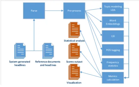
to use for the comparative evaluations. Figure 1

depicts the flowchart of the HEvAS system, with its main modules.

System generated headlines System generated

headlines

Reference documents and headlines Reference documents

and headlines

Parse Pre-process

Topic modeling LDA

Metrics calculation

Scores output Scores output

LSI Word Embeddings

POS tagging

Frequency ststistics

Visualization Visualization Statistical analysis Statistical analysis

Figure 1: HEvAS data flow

Once evaluation is finished, its results are vi-sualized at the system’s interface and written to the file system. For every headline generation sys-tem the output file (in csv format) is generated, where columns stand for chosen metrics and rows stand for the input documents. Also, one summa-rizing csv file is generated where all systems can be ranked by their avg metric scores. One sin-gle score for each system is calculated as an av-erage for every metric. Additionally, an avav-erage score over all metrics is calculated for every sys-tem; this is possible because all of the metrics are

[0,1]-normalized. Figure2shows an example of

6_{The examples of such files are provided with the}

soft-ware.

final average scores of competing systems as

gen-erated by HEvAS. Figure3shows an example of

Figure 2: Average scores over all metrics for all systems

metric average scores for the first sentence taken as a headline, generated by HEvAS.

Figure 3: All average metric scores for the first sentence system

4 Experiments

We performed experiments on a small dataset

composed of50 wikinews articles written in

En-glish7, where each document is accompanied by a

reference (gold standard) headline. The dataset is

7_{Despite the experiments were performed on English}

System/Metric R-1 R-2 R-SU R-WSU LSA-C LSA-S TM-C TM-S WE-C WE-S KL-C KL-S Random 0.046 0.000 0.011 0.018 0.869 0.721 0.783 0.586 0.693 0.445 0.593 0.954 TF-IDF 0.008 0.000 0.002 0.003 0.980 0.731 0.338 0.470 0.650 0.390 0.578 0.951 First 0.408 0.177 0.176 0.236 0.892 0.828 0.925 0.691 0.734 0.735 0.664 0.959 STextRank 0.191 0.066 0.061 0.096 0.904 0.781 0.794 0.608 0.732 0.579 0.692 0.932 WTextRank 0.263 0.009 0.082 0.114 0.857 0.768 0.923 0.663 0.735 0.613 0.719 0.906

Table 1: Mean scores of informativeness metrics.

System/Metric Fog NR PNR PR AWL Random 0.740 0.471 0.004 0.004 6.318 TF-IDF 0.786 0.511 0.000 0.000 6.853 First 0.410 0.396 0.006 0.017 5.154 STextRank 0.446 0.357 0.005 0.020 4.987 WTextRank 0.863 0.584 0.002 0.000 6.040

Table 2: Mean scores of readability metrics.

publicly available.8 Table1contains mean scores

per each informativeness metric (with default

set-tings) for all five baselines (see Section3.3). Each

metric, except ROUGE, was applied for a

cover-age (denoted byCsuffix) and a similarity (denoted

bySsuffix) scenarios. Table2contains the results

of readability metrics for all baselines.

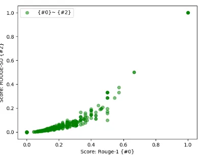
The results of a correlation analysis9 between

informativeness metrics demonstrate a high corre-lation between all ROUGE metrics and between ROUGE metrics and Word Embedding

similarity-based metric (WE-S). Figure4 shows correlation

achieved for ROUGE-1 and ROUGE-SU metrics. However, a low correlation was obtained between

Figure 4: Correlation between ROUGE-1 and ROUGE-SU metrics

all other metrics. Also, coverage metrics usually

8_{https://drive.google.com/file/d/}

1JHKH4-49UwbKdx7MIXJaLZSd444AUKFc/view? usp=sharing

9_{Performed for theF irstbaseline using Pearson}

correla-tion.

do not correlate with the similarity metrics of the

same type (an exception—correlation 0.6—was

observed in a case of TM-based metrics). There are no correlated readability metrics. The

low-est negative correlation (−0.5) was found between

AWL and Gunning Fog Index and between PNR and NR. Detailed correlation scores between dif-ferent metrics achieved for our dataset are given in

Table3.

5 Conclusions and future work

In this paper we presented a working system named HEvAS for automated headline evalua-tion. The HEvAS system provides a user with

12 metrics, where some of them are novel,

which measure headline quality in terms of informativeness—topics coverage and closeness to the human-generated headlines. Also, HEvAS provides five readability metrics, which measure

how understandable the headlines. The system

R-1 R-2 R-SU R-WSU LSA-C LSA-S TM-C TM-S WE-C WE-S KL-C KL-S R-1 - 0.74 0.99 0.99 -0.30 0.43 0.24 0.19 0.07 0.85 0.34 0.09 R-2 0.745 - 0.76 0.78 -0.16 0.35 0.07 0.07 -0.09 0.66 0.11 0.21 R-SU 0.991 0.76 - 1.00 -0.32 0.41 0.23 0.18 0.03 0.84 0.32 0.12 R-WSU 0.995 0.78 1.00 - -0.31 0.42 0.23 0.18 0.05 0.85 0.32 0.11 LSA-C -0.305 -0.16 -0.32 -0.31 - 0.28 -0.17 -0.11 -0.14 -0.21 -0.21 0.01 LSA-S 0.427 0.35 0.41 0.42 0.28 - 0.26 0.24 -0.08 0.44 -0.03 0.05 TM-C 0.237 0.07 0.23 0.23 -0.17 0.26 - 0.60 0.28 0.38 0.18 -0.03 TM-S 0.187 0.07 0.18 0.18 -0.11 0.24 0.60 - 0.11 0.28 0.06 -0.05 WE-C 0.075 -0.09 0.03 0.05 -0.14 -0.08 0.28 0.11 - 0.26 0.44 -0.39 WE-S 0.849 0.66 0.84 0.85 -0.21 0.44 0.38 0.28 0.26 - 0.29 0.00 KL-C 0.345 0.11 0.32 0.32 -0.21 -0.03 0.18 0.06 0.44 0.29 - -0.34 KL-S 0.088 0.21 0.12 0.11 0.01 0.05 -0.03 -0.05 -0.39 0.00 -0.34

-Table 3: Metric correlation scores.

References

Reinhard Bergmann, John Ludbrook, and Will PJM Spooren. 2000. Different outcomes of the wilcoxon-mannwhitney test from different statistics packages.

The American Statistician54(1):72–77.

D M Blei. 2012. Probabilistic topic models. Commu-nications of the ACM55(4):77–84.

D. M. Blei, A. Y. Ng, and M. I. Jordan. 2003. Latent dirichlet allocation. Journal of Machine Learning Research3:993–1022.

Meri Coleman and Ta Lin Liau. 1975. A computer readability formula designed for machine scoring.

Journal of Applied Psychology60(2):283.

Kevyn Collins-Thompson. 2014. Computational as-sessment of text readability: A survey of current and future research. ITL-International Journal of Ap-plied Linguistics165(2):97–135.

Carlos A Colmenares, Marina Litvak, Amin Mantrach, and Fabrizio Silvestri. 2015. Heads: Headline gen-eration as sequence prediction using an abstract feature-rich space. InProceedings of the 2015 Con-ference of the NAACL: HLT. pages 133–142.

William H DuBay. 2004. The principles of readability.

Online Submission.

Shawn Graham, Scott Weingart, and Ian Milligan. 2012. Getting started with topic modeling and mal-let. Technical report, The Editorial Board of the Pro-gramming Historian.

Robert Gunning. 1952. The technique of clear writing. .

Julia Hancke, Sowmya Vajjala, and Detmar Meurers. 2012. Readability classification for german using lexical, syntactic, and morphological features. Pro-ceedings of COLING 2012pages 1063–1080.

Yuko Hayashi and Hidekazu Yanagimoto. 2018. Head-line generation with recurrent neural network. In

New Trends in E-service and Smart Computing, Springer, pages 81–96.

Anna Huang. 2008. Similarity measures for text docu-ment clustering. Insixth New Zealand computer sci-ence research student confersci-ence (NZCSRSC2008). pages 49–56.

Lyle V Jones and John W Tukey. 2000. A sensible formulation of the significance test. Psychological methods5(4):411.

J Peter Kincaid, Robert P Fishburne Jr, Richard L Rogers, and Brad S Chissom. 1975. Derivation of new readability formulas (automated readability in-dex, fog count and flesch reading ease formula) for navy enlisted personnel .

M. J. Kusner, Y. Sun, N. I. Kolkin, and K. Q. Wein-berger. 2015. From word embeddings to document distances. InICML.

Chin-Yew Lin. 2004. Rouge: A package for automatic evaluation of summaries. InProceedings of the Text Summarization Branches Out workshop.

G Harry Mc Laughlin. 1969. Smog grading-a new readability formula. Journal of reading12(8):639– 646.

Rada Mihalcea and Paul Tarau. 2004. Textrank: Bring-ing order into text. InProceedings of the EMNLP.

Tomas Mikolov, Kai Chen, Greg Corrado, and Jef-frey Dean. 2013. Efficient estimation of word representations in vector space. arXiv preprint arXiv:1301.3781.

Jeffrey Pennington, Richard Socher, and Christopher D Manning. 2014. Glove: Global vectors for word representation. InEMNLP. ACL, volume 14, pages 1532–1543.

Luz Rello, Ricardo Baeza-Yates, Laura Dempere-Marco, and Horacio Saggion. 2013. Frequent words improve readability and short words improve under-standability for people with dyslexia. InIFIP Con-ference on Human-Computer Interaction. Springer, pages 203–219.

Shiqi Shen, Yu Zhao, Zhiyuan Liu, Maosong Sun, et al. 2016. Neural headline generation with sentence-wise optimization. arXiv preprint arXiv:1604.01904.

Sanja ˇStajner, Richard Evans, Constantin Orasan, and Ruslan Mitkov. 2012. What can readability mea-sures really tell us about text complexity. In Pro-ceedings of workshop on natural language pro-cessing for improving textual accessibility. Citeseer, pages 14–22.